Shock tube simulation project

Introduction

In this study, a shock tube simulation is set up using low and high pressure regions using Converge CFD. The results are post processed using paraview and the animations are visualized to view the effect of gaseous phase mixing.

Aim

To setup a shock tube simulation

Setup

A shock tube geometry is created using a CAD program. It is a simple geometry with two boxes, which can be defined as regions.

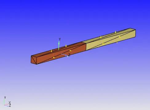
Fig. Geometry

The brown region (region 0) is initialized using a high pressure of 6e5 Pa, and the white low pressure region (region 1) using 101325 Pa.

Both regions are setup as slip walls.

In the high pressure region, N2 is setup as the material, whereas in the low pressure region, O2 is defined. The simulation is run for 0.003 s, with a minimum timestep size of 1e-7. A compressible solver is used, using a PISO formulation for the Navier Stokes equations.

The interface between the high and low pressure regions doesnt exist, meaning it is empty:

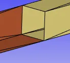Fig. Inner view between two regions showing empty interface.

The interface (made up of traingles) are deleted. Using "events" setup condition in converge, the high pressure region and low pressure regions are automatically closed and opened, where Converge forms a set of triangles as an interface (flap). In this case, at 0.001 s the event is defined as open, so that N2 at high pressure enters the low pressure O2 region.

A grid size of 0.001 m is used. The cell count is expected to increase heavily, since adaptive mesh refinement is used wherever there is a small gradient in species concentration, which is expected after the mixing of the gases in the two pressure regions.

Results

Mesh:

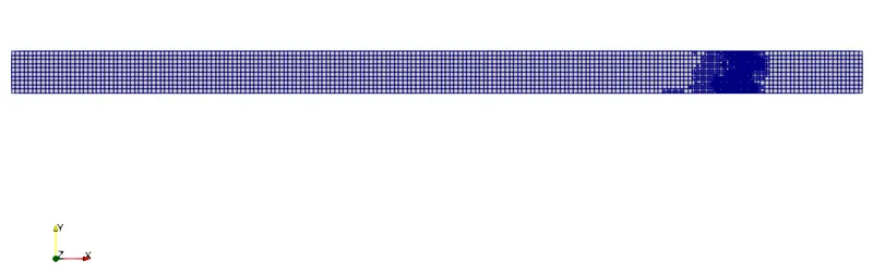
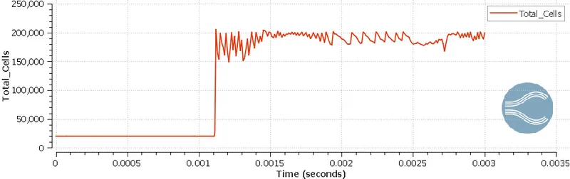
Fig. Mesh at an intermediate time step, and cell count over time.

A high increase cell conunt can be seen after 0.001 s. This is due to the opening of the flap between low and high pressure regions, leading to a variation in species concentration. This variation leads to adaptive mesh refinement, and an extremely high cell count.

Pressure and temperature variation

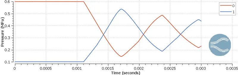
Fig. Pressure variation over time. 0 - initialized as high pressure region , 1 - intialized as low pressure region.

Here, it can be observed for region 0, there is an initial pressure drop, whereas for region 1, there is a pressure rise. This occurs after 0.001 s, when the flap is opened. Soon, however, peaks are observed, this being due to the propogation of shock waves throughout the domain during mixing of gases.

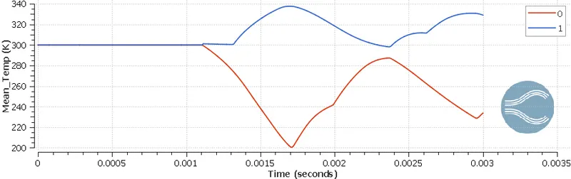
Fig. Temperature variation over time. 0 - initialized with 300 K , 1 - intialized with 300 K.

Here, it is obsevred that there are high temperature fluctuations, this is due to the heavy pressure and velocity variations, and the mixing of gases, causing the release of thermal energy.

N2 mass fraction and velocity variation with time

In this animation, it can be observed that as the fluid interacts with the right end of the solid, it moves backwards. This causes the mass fraction of N2 to keep fluctuating, w.r.t the velocity.

Conclusion

In this study, a shock tube simulation was performed using Converge CFD.