Week 7: Shock tube simulation project

SHOCK TUBE TRANSIENT SIMULATION:

AIM: To setup a transient flow simulation of a shock tube and observe the cell count as a function of time and study the temperature and the pressure contours in paraview.

THEORY: A shock tube is a simple apparatus that generates shock waves and enables flow of the fluids that are separated by the diaphragm. A shock wave inside the shock tube is created due to the high pressure that is build up in the walls of the shock tube that causes the diaphragm to open. The diaphragm is the region that separates the interface of both the fluids and prevents the diffusion or the mixing of the fluids. The burst of the shock wave creates a compression wave in the low pressure region and an expansion waves in the high pressure region. The compression waves create an increase in the pressure and the temperature in the gases. The strength of the shock waves depends upon the initial pressure ratio and across the diaphragm and the physical properties of the gases in the chamber.

PROCEDURE:

• Import the geometry in the STL file.

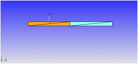
Figure 1: Shock tube geometry

• Run the diagnosis check for the geometry to check for imperfections.
• Begin the case setup
• MATERIAL: Air, Gas simulation, Global transport parameters as default.
• Simulation parameters: Transient, Full hydrodynamic and compressible.
• Simulation time parameters: 0 seconds to 0.003 seconds
• Turbulence kept as default RNGk –epsilon.
• Base grid as 0.001m
• Region and initialisations: Two regions created namely high (species N2) and the low pressure (Species O2) region.

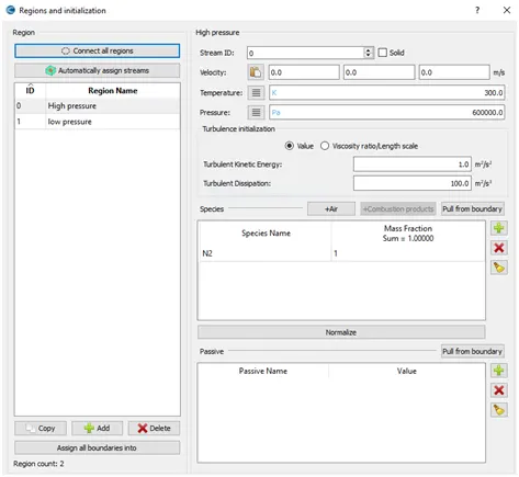
Figure 2: Regions and initialization

• Events: Events created to indicate the opening of the diaphragm. At 0 seconds it is closed and at 0.001 seconds it is open from the high pressure region to the low pressure region.

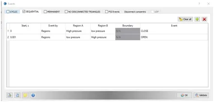
Figure 3: Events

11) Adaptive Mesh refinement: For a species of 0.001 and 3 level of embed.

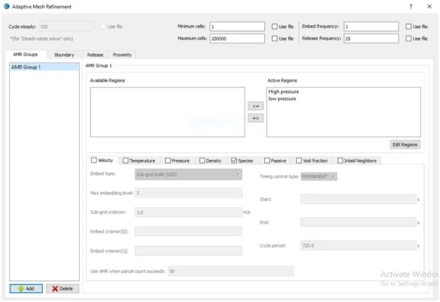
Figure 4: AMR

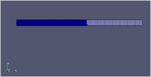
Figure 5: Mesh geometry with species based AMR

• After setting up the case export the input files in a folder to process the output and open the file in paraview to view the results.

OBSERVATION:

PRESSURE CONTOUR:

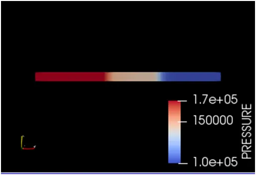
Figure 6: Pressure contour

The pressure inside is kept as 600000pa and the low pressure as 101325pa. When the diaphragm breaks the high pressure waves and the low pressure waves are reflected back and forth. Thus the shock waves which flow in supersonic speeds form an expansion fan with infinite number of shock waves.

TEMPERATURE CONTOUR:

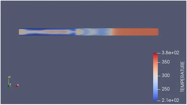
Figure 7: Temperature contour at 13 cycles

Due to the reflection of the high pressure and the low pressure waves the temperature will vary directly W.R.T to the pressure difference between the gases at the chamber.

CELL COUNT AS A FUNCTION OF TIME:

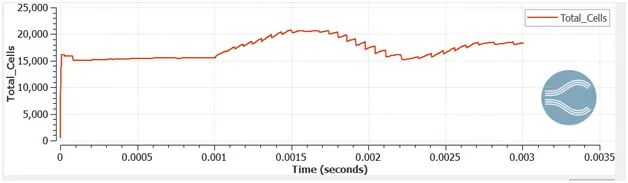
Figure 8: Total Cell count vs. time

The cell count is changing due to the adaptive mesh refinement feature based on species that we have given. As the diaphragm opens the shock waves are produced N2 from the high pressure region will disperse into the low pressure region which will cause the mesh to become finer. This process i.e. the mesh becomes finer as a result of which the cell count will increase takes place until an equilibrium is obtained, when both the gases are finished diffusing and an uniform pressure is obtained in the shock tube.

CONCLUSION: The concept of shock wave was studied successfully using AMR and events feature in converge studio. The youtube links for the temperature and the pressure contours are given below.

Temperature contour: https://youtu.be/sEDnQOSZ8O4

Pressure contour: https://youtu.be/llIwRAKV3eY