Week 6: Conjugate Heat Transfer Simulation

CONJUGATE HEAT TRANSFER SIMULATION

AIM: To setup a conjugate heat transfer case for a cylinder and post process in paraview for 3 different super cycling time intervals and base grids.

THEORY: Conjugate heat transfer (CHT) simulation takes place where heat transfer occurs simultaneously within and between the fluid and the solid region. This CHT analysis takes place where the flow happens in a pipe or the interface between the solid and the fluid region and the heat is transferred by conduction or convection. Converge solves fluid heat transfer by energy equation and the solid part by solid heat equation which is given below. Real life applications of CHT includes

-heat transfer from the engine block to the coolant

-Engine block heating due to combustion.

- Forced convection cooling of engine blocks.

- Gas turbines.

C_p𝞀= 𝞩.(K.𝞩T)(Heat flux due to conduction)+ S_h( Volumetric heat source)

SUPERCYCLING: Super cycling is a method used in converge CFD mostly for problems involving multi phase regions i.e. a solid and a fluid region or mainly used in combustion problems. If a steady state or a transient based solver is used for the both the solid and fluid it will take ages to complete the simulation and the values will probably never converge. A super cycling time control uses a transient solver for the fluid and a steady state solver for the solid region. The transient solver solves both the solid and fluid for some characteristic time and then and then the fluid solver is frozen, further the steady state solver solves both the solid and the fluid and the fluid solver is unfreezed. The process continues until the values are converged.

Y+: Wall functions are useful to tell solver how to approach the solution near the wall or the surface that helps in predicting the boundary conditions at the surface for a turbulent flow. Y+ value does not affect laminar flow. In a turbulent flow we can divide the boundary layer into three sub domains

The inner layer or sub layer where viscous shear dominates

The outer layer or the viscous shear layer where the flow is supposed to take place.

The log layer where the velocity profiles have a logarithmic variation.

To capture the effects under the viscous shear layer Y+ helps us. It is a non dimensional number that can be used to understand whether the boundary conditions are fine or not. Y+ value should mostly lie between 0 and 10 and or greater than 30. If we get a y+ value of 15 it means that our simulation is incorrect even though it has converged it may not show the accurate values and plots. In such cases we might have to look for errors in boundary condition such as no slip or law of the wall boundary condition.

PROCEDURE:

• The geometry For the simulation is sketched in converge CFD and the boundaries are flagged namely inlet, outlet, solid outer wall , interface and the solid side.
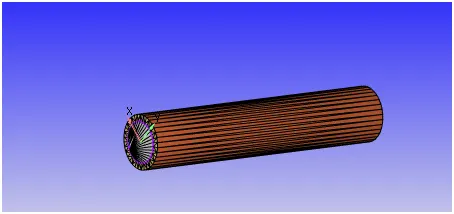
• Figure 1: Geometry

The case setup is done by selecting the various inputs such as

1. The material for the solid region is selected as aluminium and is under the solid simulation tab
2. Simulation parameters such as the selection of transient solver setting up the simulation start time and the end time, sample size are given as inputs.

• The initial conditions for the 2 regions i.e. solid and the fluid regions are given under the regions and initialisation tab.

1. The boundary condition for all the flagged regions are given such as for solid outer wall boundary a heat flux of -10000W/m² is given. Note that the negative heat flux implies that the heat flows into the system. And the pressure for the outlet is given as 1010325Pa and for the interface, 2 sets of boundary conditions are given.

• Forward boundary: A forward region specifies the forward direction of motion i.e. towards the outlet of the cylinder is called the forward boundary. Hence fluid region is selected as the forward region and the temperature and the velocity are given.
• Reverse boundary condition: An exact contrary to the forward region. Solid region is selected as the reverse region and the velocity and the pressure is given.

1. In physical models super cycling is selected and the various inputs to it such as the begin super cycle storing data and the time interval are given.

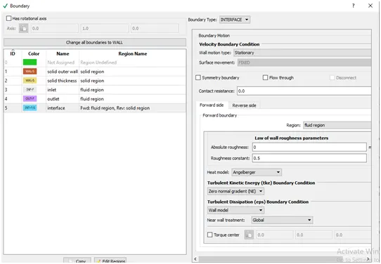
Figure 2: Interface BC

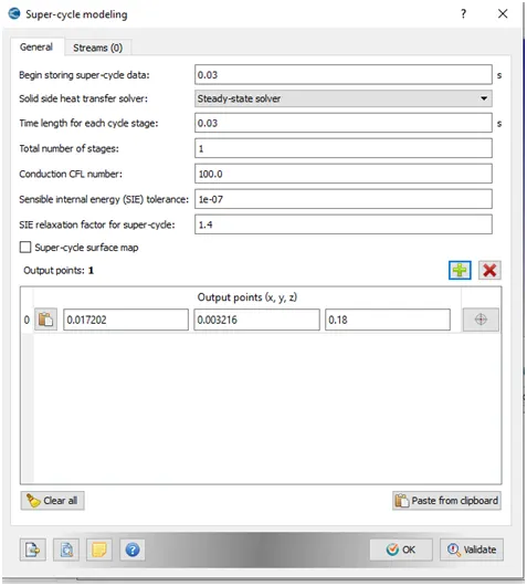
Figure 3: Super cycling model

1. VI) The base grid for the meshing is given as 0.004m

VII) The output and the post processing inputs are specified.

• The input files are generated to a folder
• The input files are run using the executable files and the output files are then post converted
• The post converted files are opened in paraview and several properties are viewed under investigation
• The method is repeated for different super cycling time intervals i.e. 0.01, 0.02 and 0.03 and different base grids.

OBSERVATION:

FOR BASE GRID SIZE 0.004 and super cycling interval 0.001

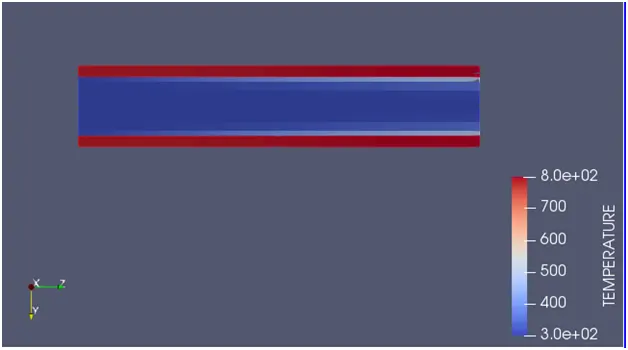
Figure 4: Temperature contour

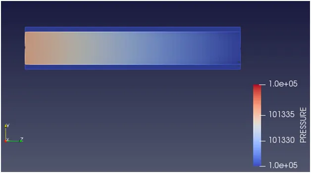
Figure 5: Pressure contour

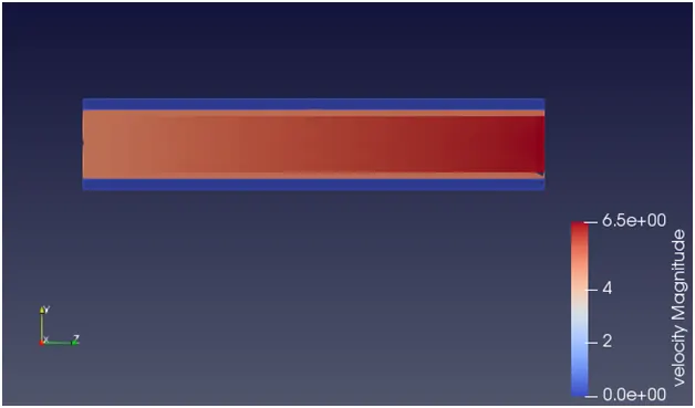
Figure 6: velocity contour

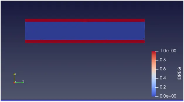
Figure 7: ID region- red for solid and blue for fluid

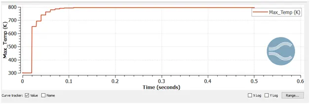
Figure 8: Max temperature under super cycling

CASE 2: for a base grid of 0.003 and super cycle interval of 0.02 seconds

Figure 9: Velocity contour

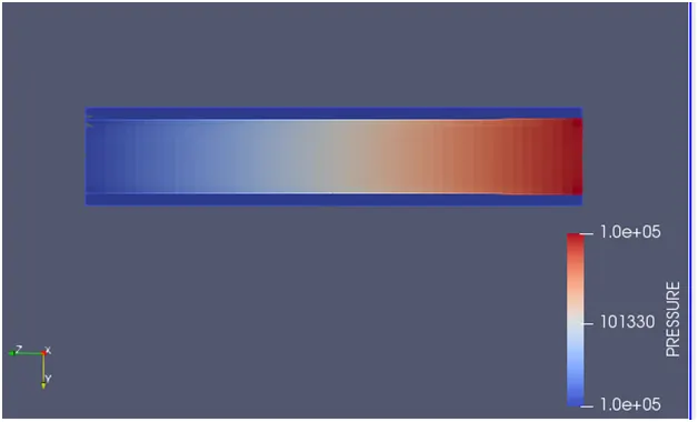
Figure 10: Pressure contour

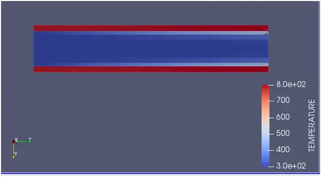
Figure 11: Temperature contour

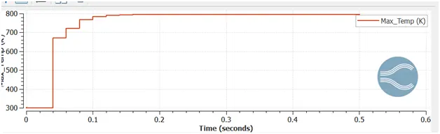
Figure 12: Max temperature

CASE3: For a base grid of 0.002 and super cycling interval of 0.03

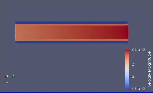
Figure 13: Velocity contour

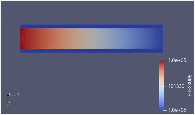
Figure 14: Pressure contour

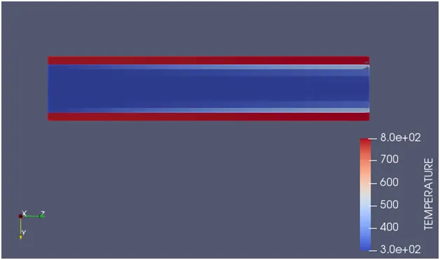
Figure 15: Temperature contour

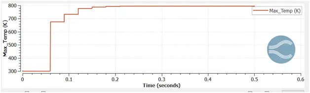
Figure 16: Max temperature

CONCLUSIONS: The temperature of the fluid increases due to the increase contact with the pipe and heat flux is given as an input which causes an increase in temperature across the diameter of the pipe.The pressure takes a decreasing legend as the flow takes place from a region of higher pressure to lower pressure. As far as the super cycling model is concerned, we can say when the super cycling interval increases the solution converges at a slower rate. Hence the computational time increases since the time taken reach the steady state value increases but, the final values remain the same