Week 7: Shock tube simulation project
Aim: To set up transient shock tube simulation.
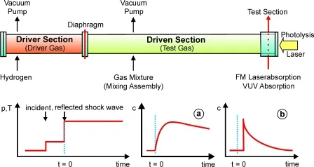
Introduction: The shock tube is an instrument used to replicate and direct blast waves at a sensor or model in order to simulate actual explosions and their effects usually on a smaller scale. They are also used to study combustion and chemical kinetics at high temperatures and pressure. A shock tube generates a shock wave using sections of high-pressure and low-pressure gas separated by a diaphragm. when the diaphragm ruptures the driver and driven gas come in contact with each other creating a contact surface that acts as a piston compressing the test gas in the driven section. The shock wave travels through the diven section hits the end wall and reflects back this causes further compression of test gas and stagnates it.
Procedure:
To create / import geometry:
1) click on file > import > import STL then select the path of .STL file to be imported and click import.
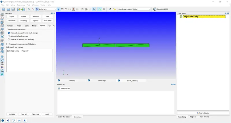
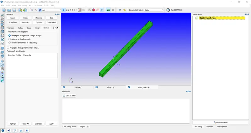
2) Click on diagnosis to check for any errors. If all the normals are pointing inside the geometry then we can move ahead if not we can flip the orientation of normals inside using Transform > Normals > Propogate change from single triangle select a triangle and hit apply.
3) Next step is the boundary creation
Case Set up:
1) Click on begin case set up to start case set up select application type as time-based and Predefined mixture as the air. Uncheck reaction mechanism and check species.
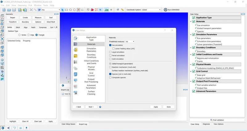
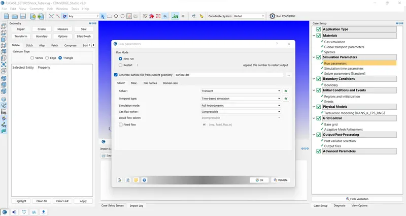
2) Do not change global transport properties and add species N2 and O2 in the species section, In run parameters select solver type to be the transient state solver.
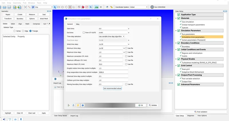
3) In simulation time parameters start time is 0 sec and the end time to be 0.003 sec initial time step is 1e-9 secs, the minimum time step is 1e-9 sec and the max time step is 1 sec.
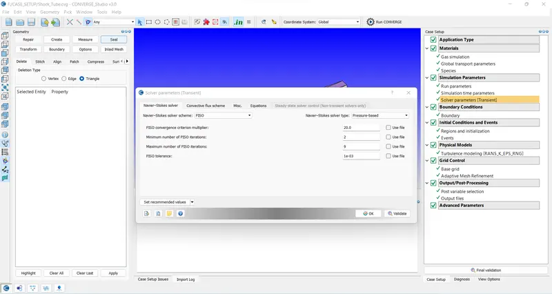
4) In solver parameters select Navier-stokes solver type as the pressure-based solver.
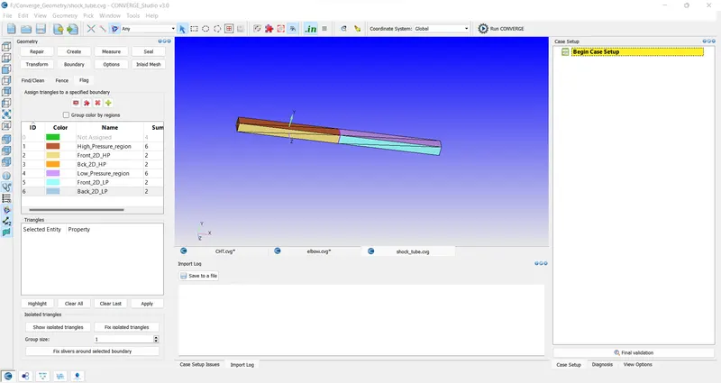
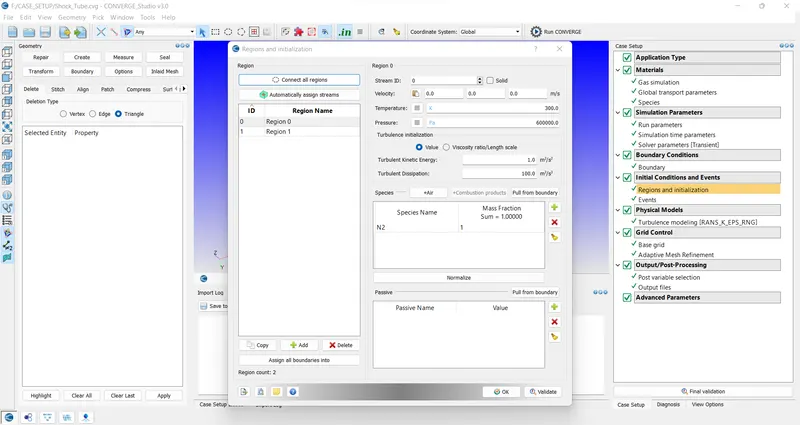
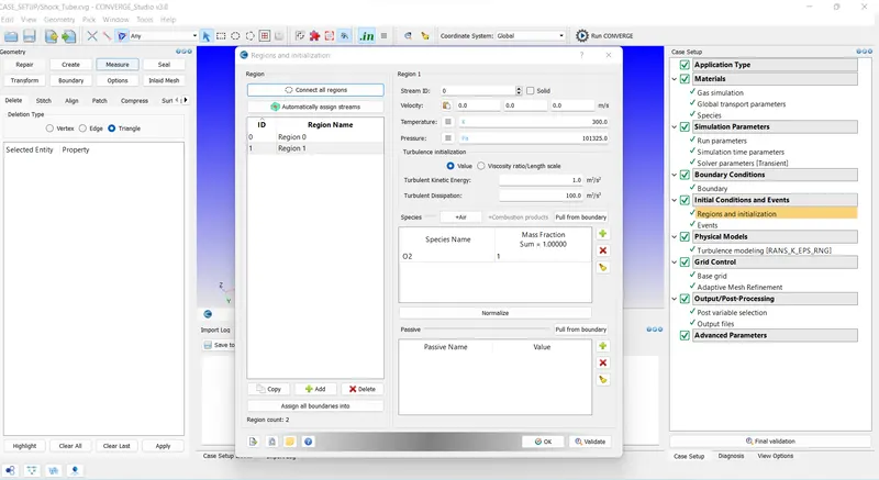
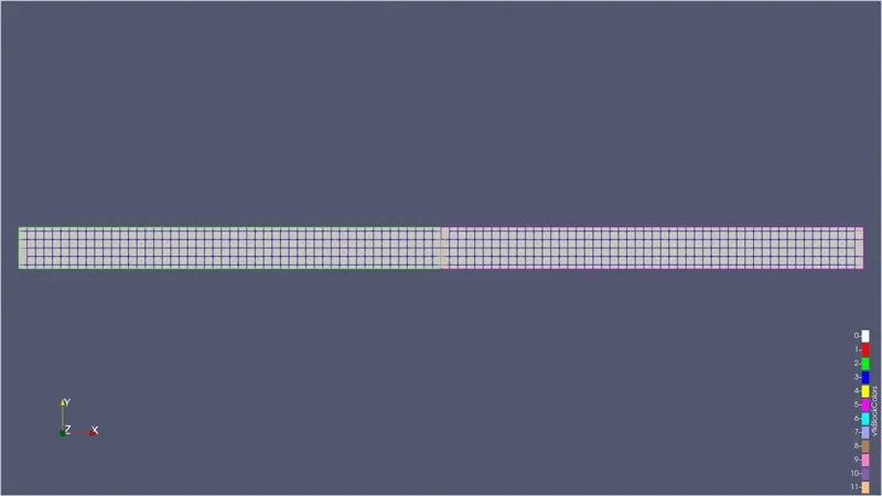
5) Add two regions Region0 as the high-pressure region and Region1 as the low-pressure region. Region0 is only N2 species and Region1 is O2 species. Pressure in Region0 is 6bar and in Region1 is 1 atm.
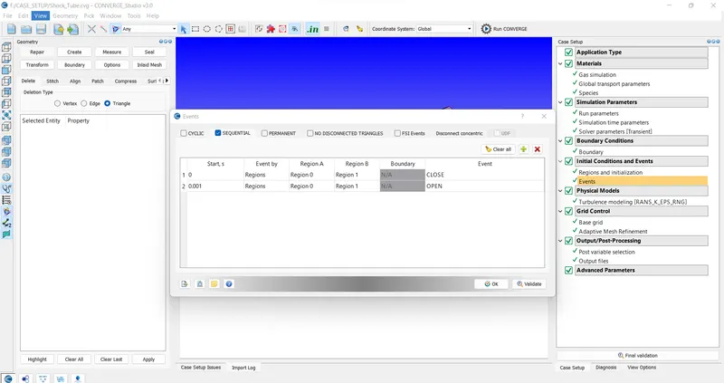
6)In Initial condition and Events add event> Sequential> both reagions are closed till 0.001 sec after 0.001 sec the regions are open.
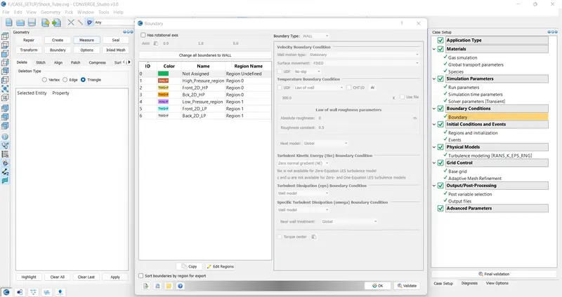
7) In boundary assign boundaries as follows:
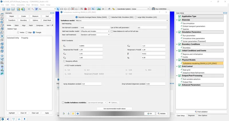
8) In the Physical model select RNG k-εε keeping other values as default.
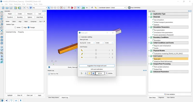
9) Create 3 different mesh sizes as 0.001m 0.002m and 0.003m.
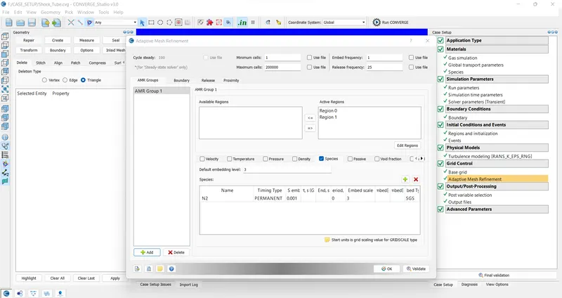
10) From grid control add AMR. In AMR use species to based AMR use permanent AMR and embed scale is 3. Add both regions to active regions.
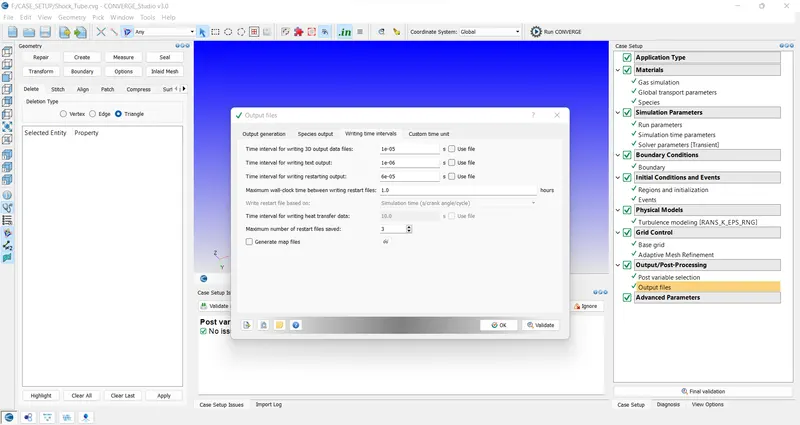
11) In output files time interval for writing 3D output file to be 1e-5 sec and time interval to write Text output file to be 1e-6 dec. Do not change anything in post-variable selection. Click on final validation to check for any errors.
Processing input files:
1) Click on file > export > input files
2) Copy and paste licence.lic and mpiexec.exe file in the folder of input files
3) Open Cygwin browse to input files folder
4) Enter the following commands
mpiexec.exe -n 6 “C:\Program Files\Convergent_Science\CONVERGE\3.0.16\bin\intelmpi\converge.exe” restricted
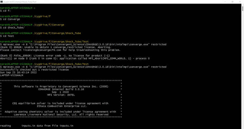
5) After completion of the process.
6) Copy and paste the post_convert file in the output folder in the cygwin Enter command
mpiexec.exe -n 6 post_convert
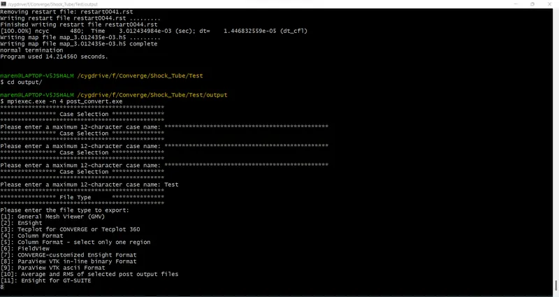
7) Enter the Name for the case selection
8) Enter file type to export as Paraview VTK in-line binary format
9) Select yes to put boundary surface output
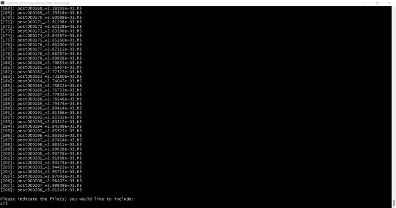
10) Include all file for post processing
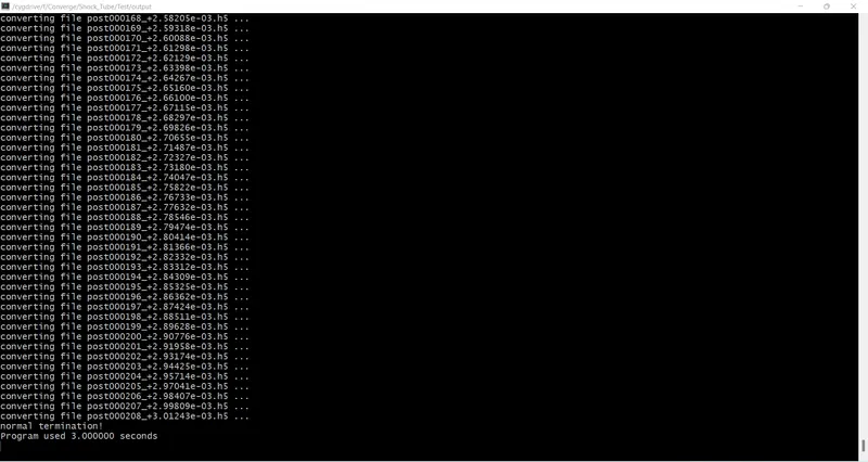
11) Include all cell variables
Post-processing of files:
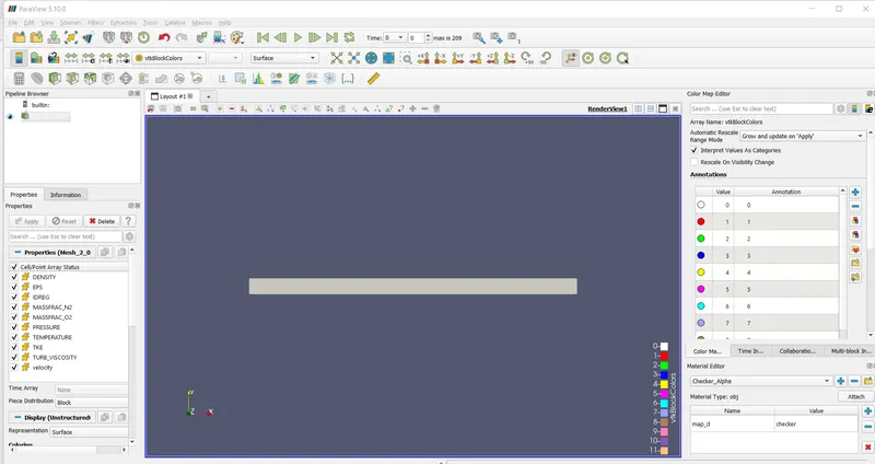
1) Open Paraview for post-processing and open a folder named output and open the file with extension .vtm and click apply.
2) Click on slice and along Z normal uncheck triangulate slice and show plane.
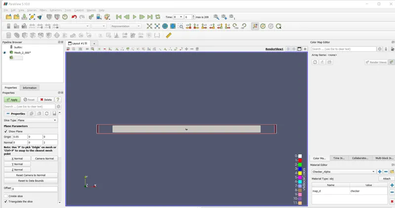
3) Select velocity click play and check on visibility change.
Results:
Mesh_1
Grid Size=0.001m
Pressure History
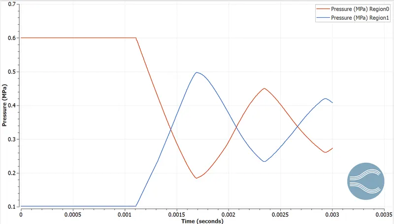
Pressure in both boundaries will remain constant till 0.001sec after that the regions will mix. the fluid in region0 will expand so the pressure is reduced. Fluid in the region1 will compress. after the shock wave reflects N2 will again compress so the pressure in region 1 is seen to be increased again.
Temperature History
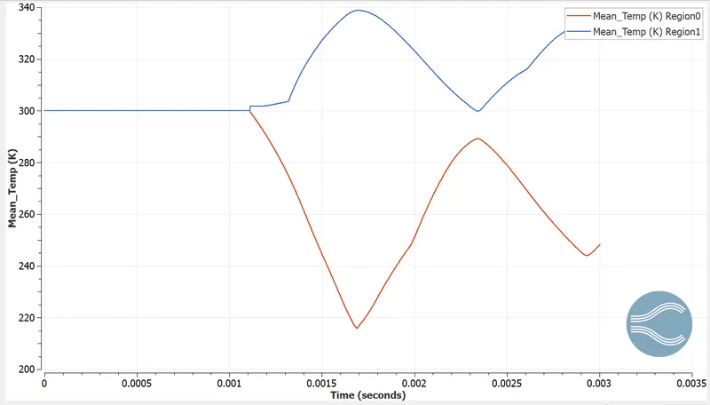
In region0 as the fluid is at high pressure after the opening of the boundary N2 in region0 will expand so the temperature will drop. After some time the shock wave will reflect compress the N2 so the temperature will increase.
cell count:
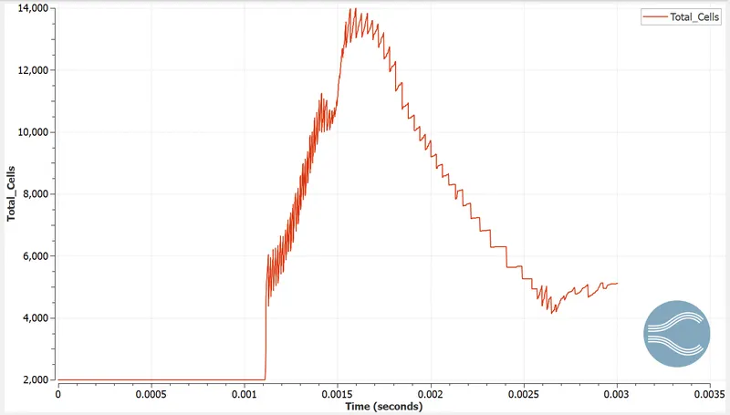
After 0,001 sec the regions are open so they start interacting and due to AMR of the species. at their boundary mesh is refined. hence the cell count is high after 0.001 sec.
Mesh_2
Grid size =0.002m
Pressure history:
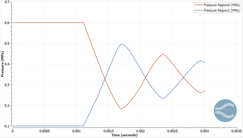
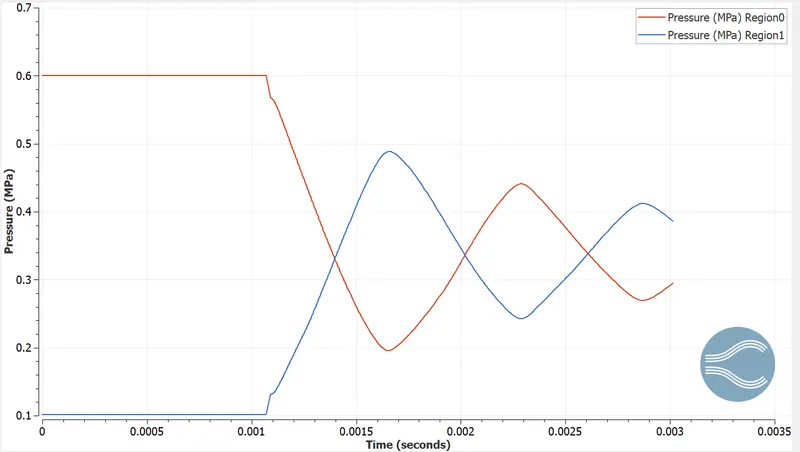
Pressure in both boundaries will remain constant till 0.001sec after that the regions will mix. the fluid in region0 will expand so the pressure is reduced. Fluid in the region1 will compress. after the shock wave reflects N2 will again compress so the pressure in region 1 is seen to be increased again.
Temperature History
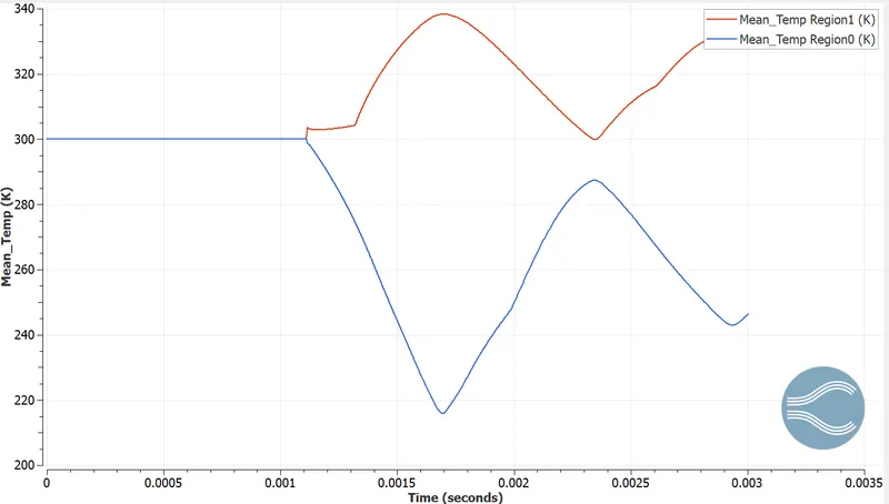
In region0 as the fluid is at high pressure after the opening of the boundary N2 in region0 will expand so the temperature will drop. After some time the shock wave will reflect compress the N2 so the temperature will increase.
Cell count:
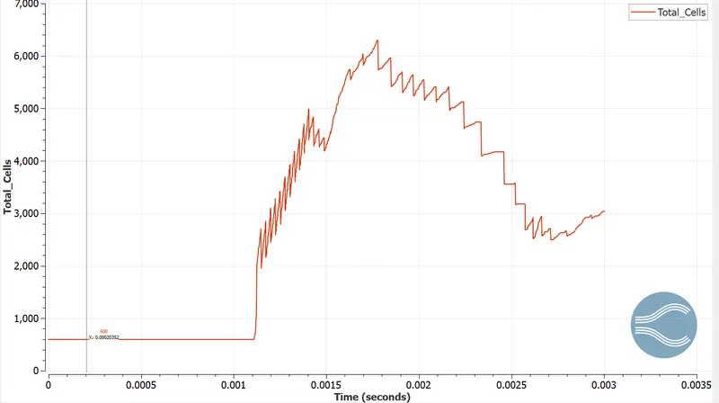
After 0,001 sec the regions are open so they start interacting and due to AMR of the species. at their boundary mesh is refined. hence the cell count is high after 0.001 sec.
Mesh_3
Grid Size=0.003m
Pressure history:
Temperature history:
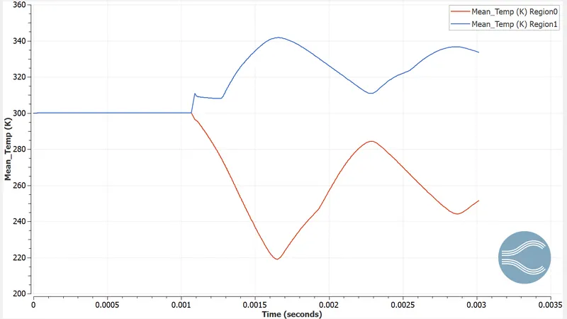
In region0 as the fluid is at high pressure after the opening of the boundary N2 in region0 will expand so the temperature will drop. After some time the shock wave will reflect compress the N2 so the temperature will increase.
Cell Count
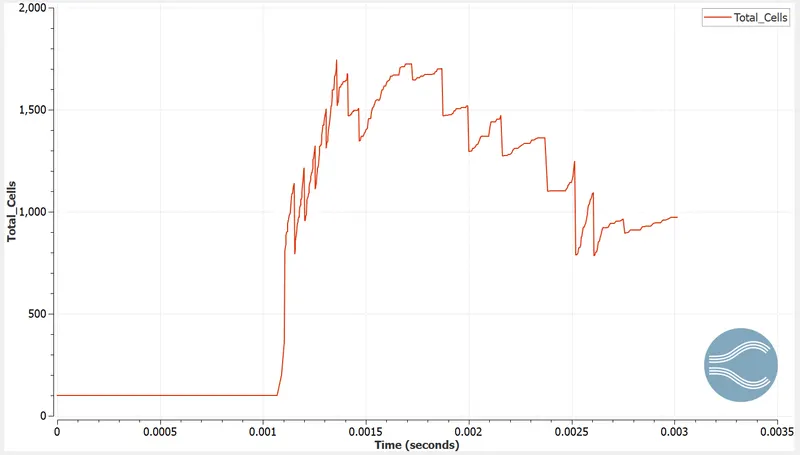
After 0,001 sec the regions are open so they start interacting and due to AMR of the species. at their boundary mesh is refined. hence the cell count is high after 0.001 sec.
AMR: https://youtu.be/WcC_1tXima0
Species:https://youtu.be/dUyI8rd3fFg
Pressure:https://youtu.be/_gRoiUr96h0
Temperature:https://youtu.be/XV6VCsbiDik
Velocity:https://youtu.be/JY0gRcKyqJ4