Week 6: Conjugate Heat Transfer Simulation
Aim: To set up flow simulation through a pipe for studying conjugate heat transfer.
Introduction:
Conjugate Heat Transfer:
Heat transfer is an exchange of thermal energies between two bodies at different temperatures. this rate is directly proportional to the temperature difference between these two bodies.
Conjugate heat transfer is a type of heat tranfer analysis between solids and fluids which includes both conduction and convection heat transfer processes.
At 300K and 1atm properties of air are given below
Density=1.161Kg/m^3
Dynamic viscosity= 1.846*10^-5
Diameter of pipe=0.03
Re=7000
`Re=\frac{\rho v D}{\mu}`
v=3.71m/s^2
Procedure:
To create / import geometry:
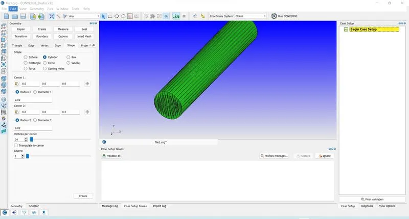
1) Click on Create>Shape>Cylinder
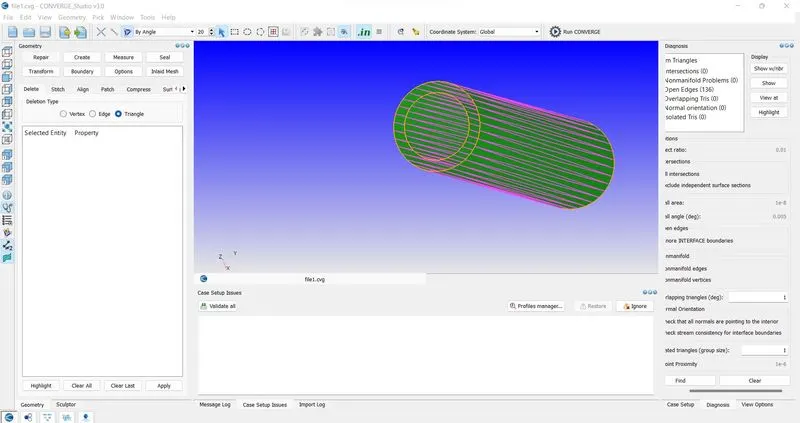
2) after creating the cylinder delete intersecting triangles by clicking on Repair>Delete> by surface selection select the intersecting triangles and click apply.
3) Create boundaries to represent the thickness of the solid and volume of fluid. Seal the open edges using create>triangles>loft edges select two edges and click apply.
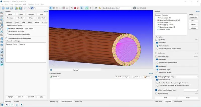
4) Flip normals if they are pointing in the wrong direction.
Case Set up:
1) Click on begin case set up to start case set up select application type as time-based and Predefined mixture as the air also check on solid simulation as solid is involved in this simulation. Uncheck reaction mechanism and check species.
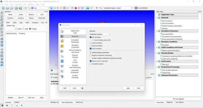
2) Do not change global transport properties. add species N2 and O2 for gas and for solid add aluminum, in the species section.
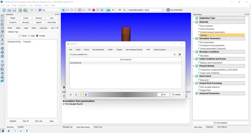
3)In run parameters select the solver type to be the transient-state solver.
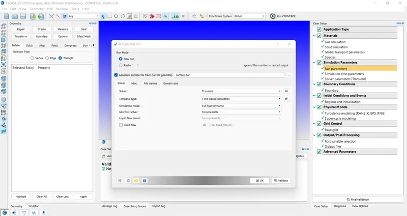
4) In simulation time parameters start time is 0 sec and the end time to be 0.5 sec initial time step is 1e-7 secs, the minimum time step is 1e-7 sec and the max time step is 1 sec.
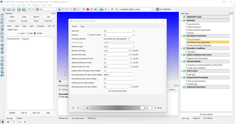
5)In solver parameters select the Navier-stokes solver type as a Density-based solver.
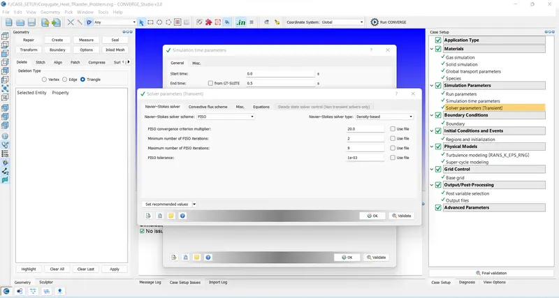
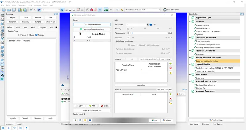
6) Add two regions solid and fluid. For solid region set stream ID to 1 and check solid flag. species as Aluminum and mass fraction as 1.0.
7) Set up boundary conditions for each of them.
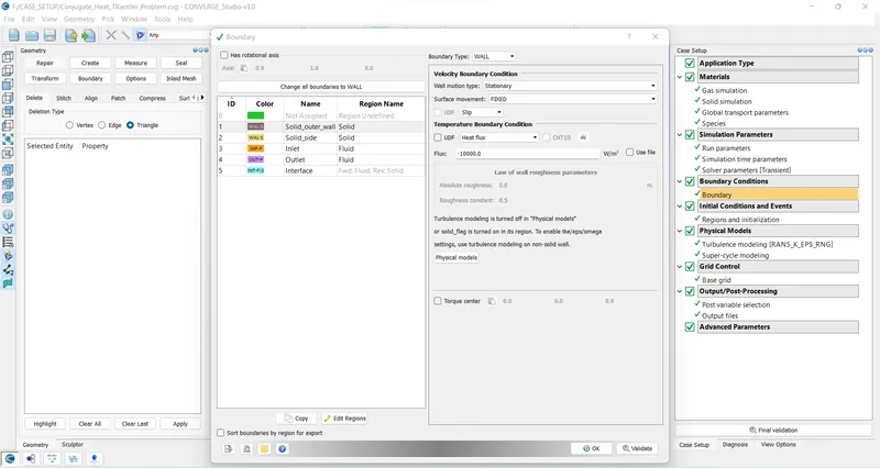
Solid outer wall - Wall -stationary wall
slip wall
Temperature : -10000W/m^2
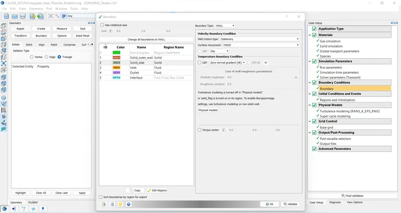
Solid side- Wall - stationary wall
Slip wall
Temperature: zero normal gradient
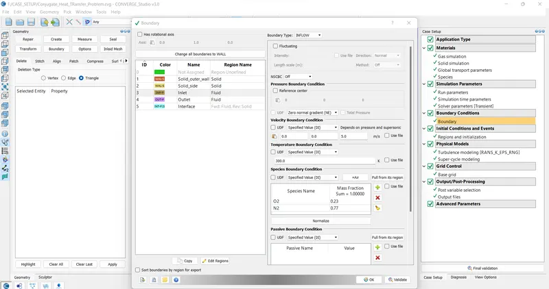
Inlet - Inflow boundary condition
Pressure: Neumann boundary Condition
Velocity along z direction: 5m/s
Outlet- Outflow
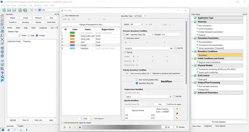
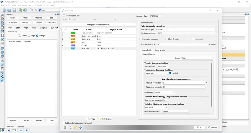
Interface- interface type boundary condition
Forward: Fluid Region
Law of wall
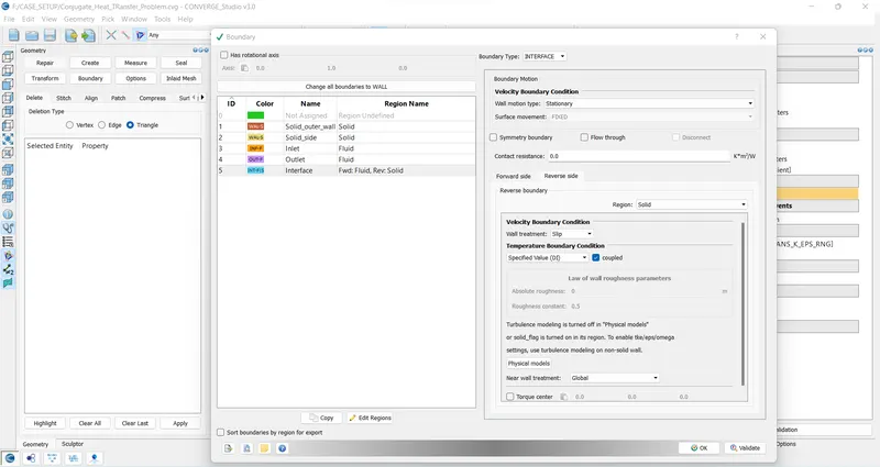
Reverse: Solid
Slip
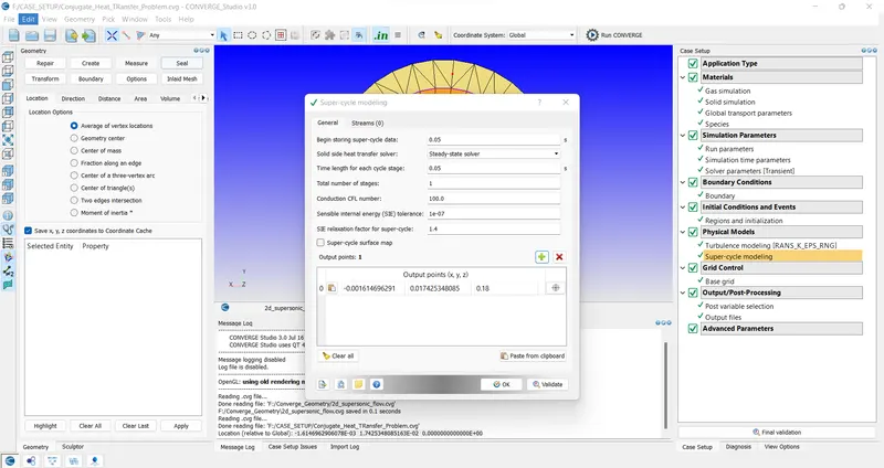
8)In the Physical model select RNG k-εε keeping other values as default. Click on super cycling.
start at 0.05sec
time length for each step is 0.05sec
add monitorpoints ponts where you want to measure the temperature
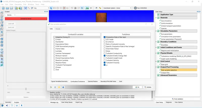
10) In post-variable selection under combustion/turbulence click on y+
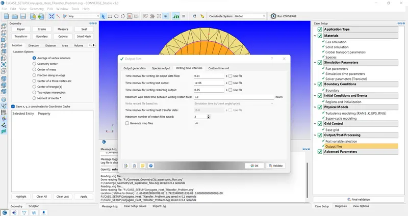
11) For output files
set write 3-D output after every 0.01 sec
write text output after every 1e-6 sec
Processing input files:
1) Click on file > export > input files
2) Copy and paste licence.lic and mpiexec.exe file in the folder of input files
3) Open Cygwin browse to the input files folder
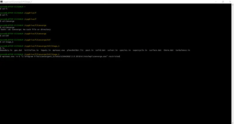
4) Enter the following commands
mpiexec.exe -n 6 “C:\Program Files\Convergent_Science\CONVERGE\3.0.16\bin\intelmpi\converge.exe” restricted
5) After completion of the process.
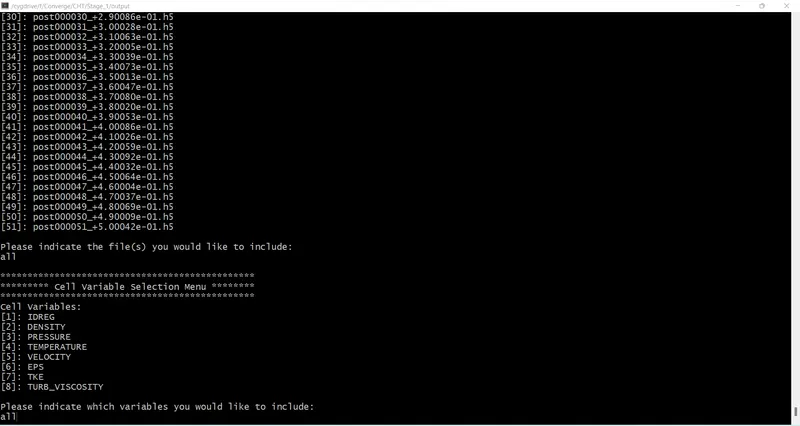
6) Copy and paste the post_convert file in the output folder in the cygwin Enter the command
mpiexec.exe -n 6 post_convert
7) Enter the Name for the case selection.
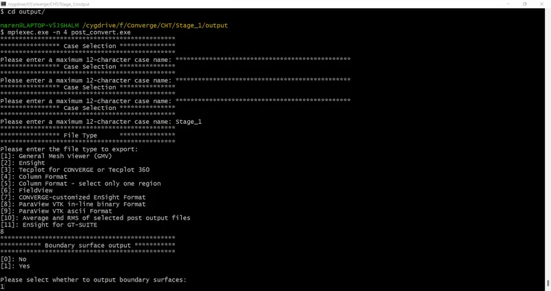
8) Enter file type to export as Paraview VTK in-line binary format
9) Select yes to put boundary surface output
10) Include all files for post-processing
11) Include all cell variables
Post-processing of files:
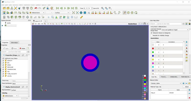
1) Open Paraview for post-processing and open a folder named output and open the file with extension .vtm and click apply.
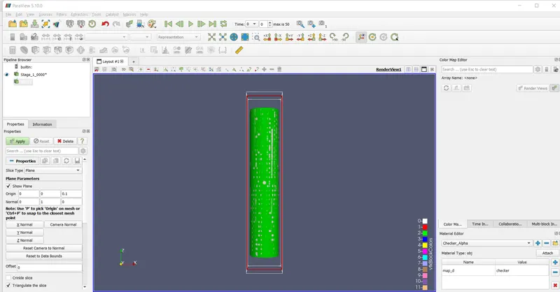
2) Click on the slice and along Y normal uncheck triangulate slice and show plane.
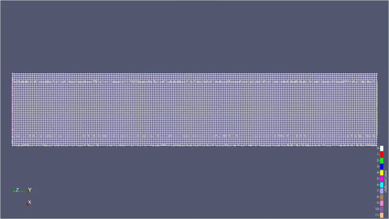
3) Select velocity click play and check on visibility change.
Result:
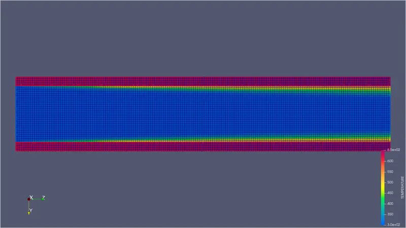
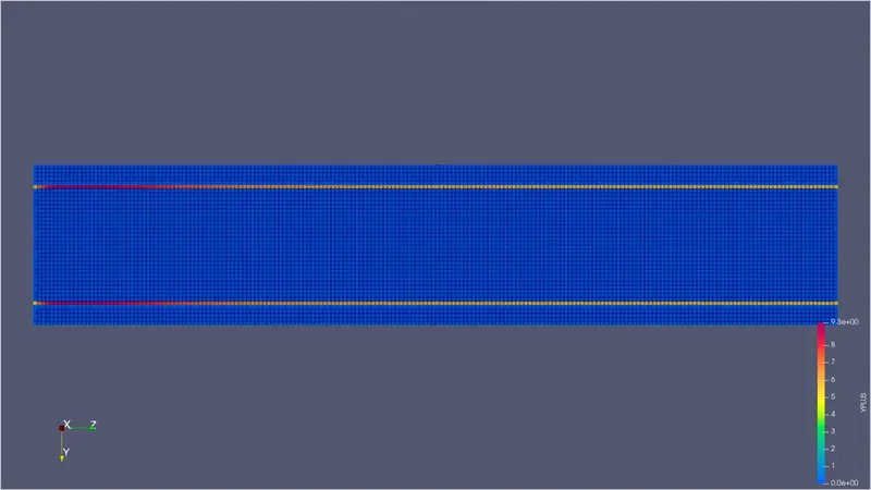
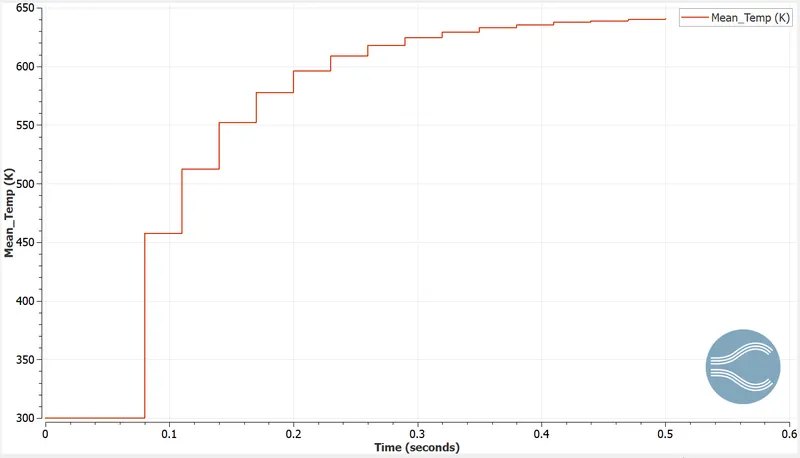
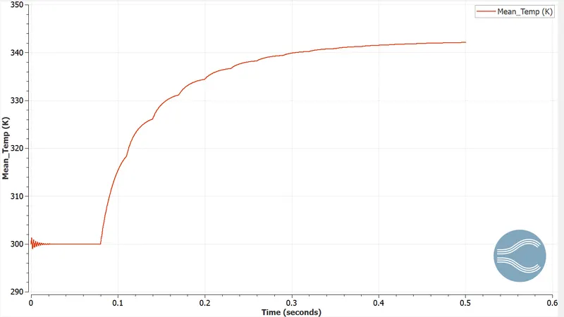
Mesh-1
Grid size=0.001m
Temperature distribution:
Y+value
Temperatureconserve in solid region
Temperature conserved in fliued region:
YouTube:
Mesh-2
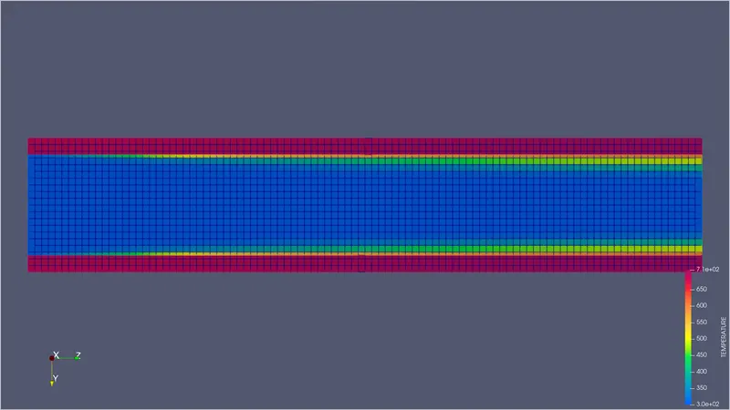
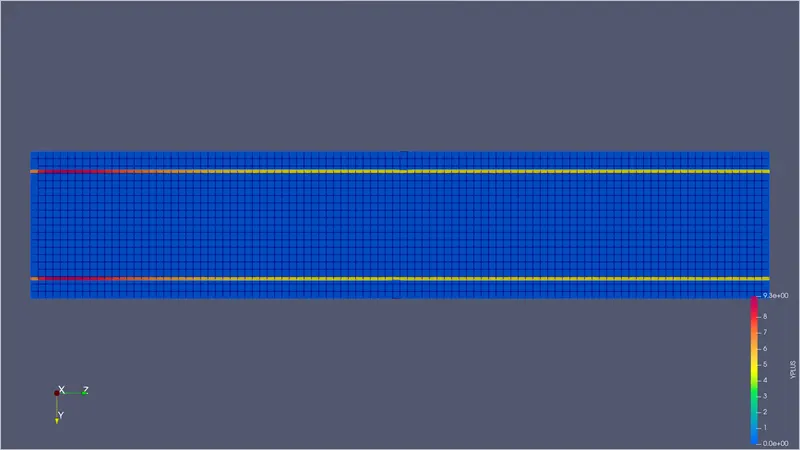
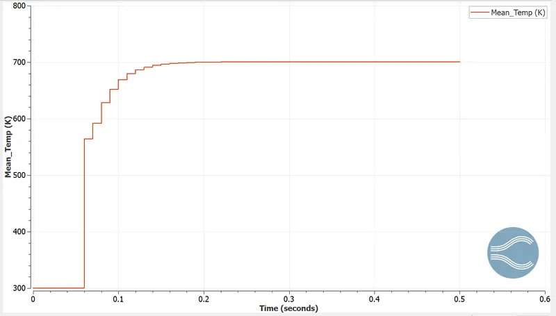
Grid size=0.002
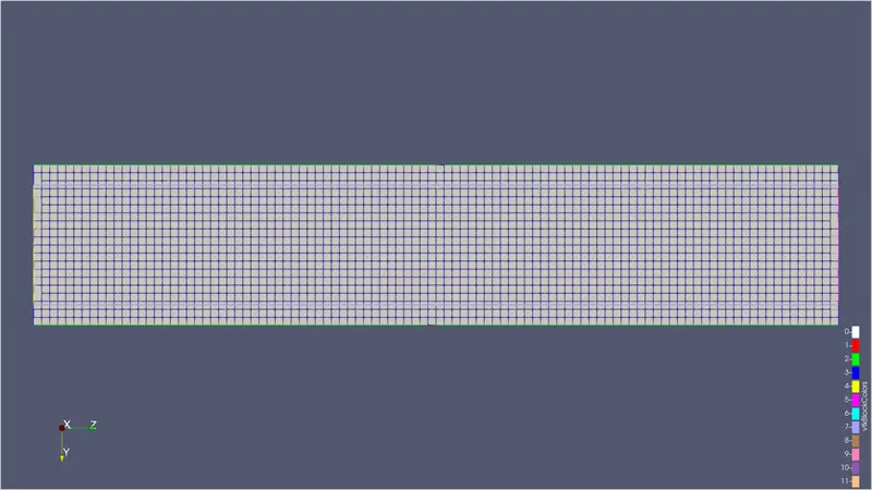
Temperature distribution:
Y+ value:
Temperature in solid region converges to
The temperature in fluid region converges to
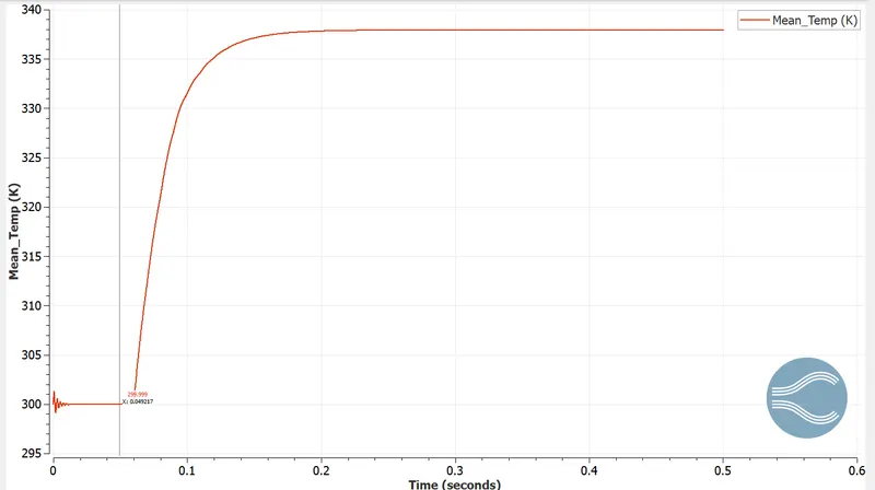
YouTube:
Mesh-3:
Grid size=0.003
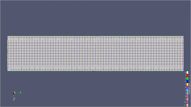
Temperature distribution:
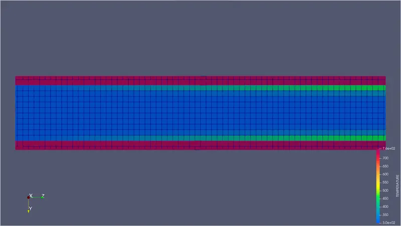
Temperature (solid region):
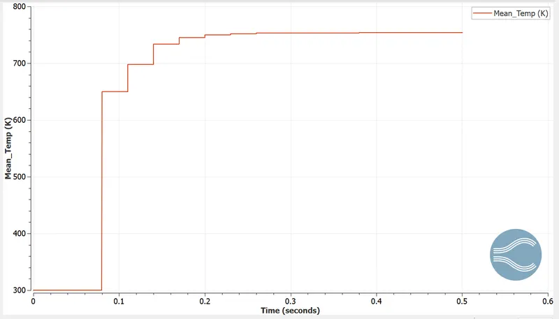
Temperature (fluid region):
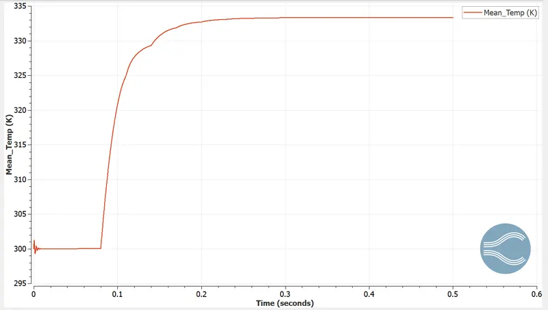
YouTube:
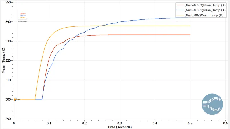
Temperature (fluid region)
Temperature (solid region)
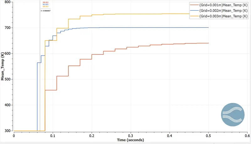
| Grid size | Temperature(Fluid Region) | Temperature(Solid Region) |
| 0.001 | 342K | 639K |
| 0.002 | 337K | 700K |
| 0.003 | 333K | 753K |
Super-cycling stage temperature
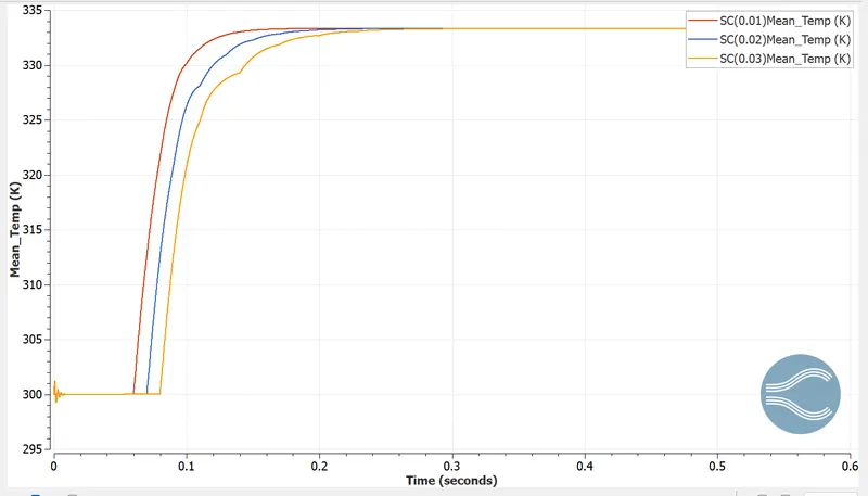
| Stage Interval | Time |
| 0.01 | 344 sec |
| 0.02 | 363 sec |
| 0.03 | 376 sec |