Week 5: Prandtl Meyer Shock problem
Aim: To perform simulation of the Prandtl Meyer shock problem.
1) Boundary conditions used for shock flow problems:
i)Neumann boundary conditions: It is the Second type Boundary condition or The Neumann boundary condition define the value of a normal derivative of a function on the surface. dy/dn = f(t).The normal derivative of the dependent variable is specified on the boundary.
ii)Cauchy boundary conditions: Both the value and the normal derivative of the dependent variable are specified on the boundary.
iii)Robin boundary conditions: It is the third type boundary condition also known as the Fourier type condition. The value of a linear combination of the dependent variable and the normal derivative of the dependent variable is specified on the boundary.
iv)Dirichlet boundary conditions: It is the first type of boundary condition. The Dirichlet boundary condition define the value of a function itself on the surface i.e. Y = f(t). The value of the dependent variable is specified on the boundary. The no-slip condition for viscous fluids states that at a solid boundary, the fluid will have zero velocity relative to the boundary.
2) What is Shock Wave?
A shock wave occurs when the speed of the moving object in a medium exceeds the speed of the sound, then the wavefronts lag behind the object forming a cone-shaped region with the source at the Vertex behind the object. The edge of the cone forms a supersonic wavefront with a large amplitude which is called a Shock wave.
Across a shock wave, the static pressure, temperature, and gas density increase almost instantaneously. The changes in the flow properties are irreversible and the entropy of the entire system increases. The total pressure downstream of the shock is always less than the total pressure upstream of the shock; there is a loss of total pressure associated with a shock wave.
3) Effect of SGS parameters on shock location:
Procedure:
To create / import geometry:
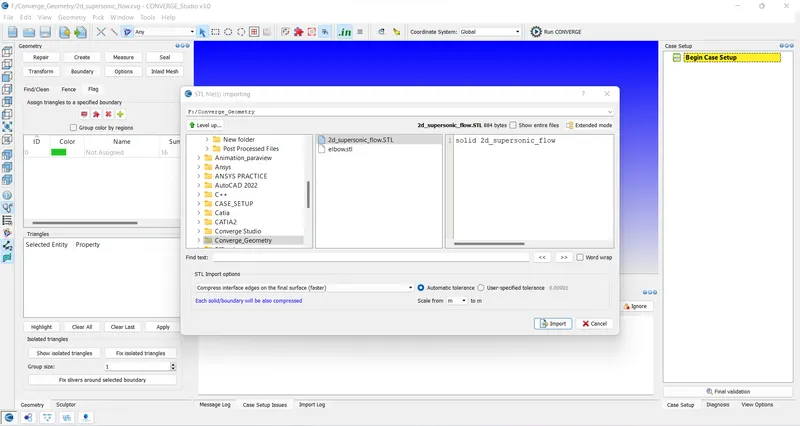
1) click on file > import > import STL then select the path of .STL file to be imported and click import.
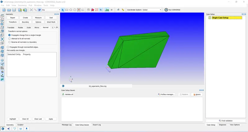
2) Click on diagnosis to check for any errors. If all the normals are pointing inside the geometry then we can move ahead if not we can flip the orientation of normals inside using Transform > Normals > Propogate change from a single triangle select a triangle and hit apply.
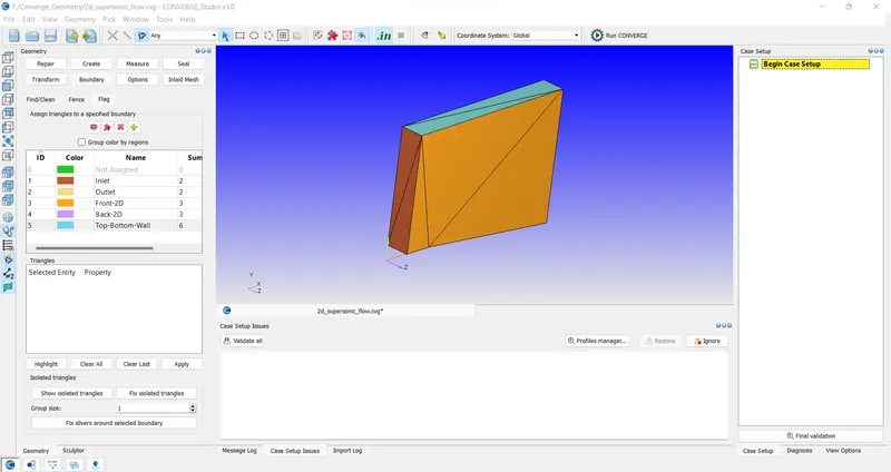
3)Next step is boundary creation.
Case Set up:
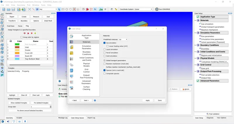
1) Click on begin case set up to start case set up select application type as time-based and Predefined mixture as the air. Uncheck reaction mechanism and check species.
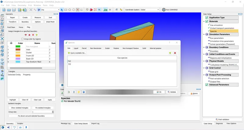
2) Do not change global transport properties and add species N2 and O2 in the species section, In run parameters select solver type to be the steady-state solver.
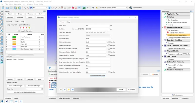
3) In simulation time parameters start time is 0 cycles and the end time to be 25000 cycles initial time step is 1e-9 secs, the minimum time step is 1e-9 sec and the max time step is 1 sec.
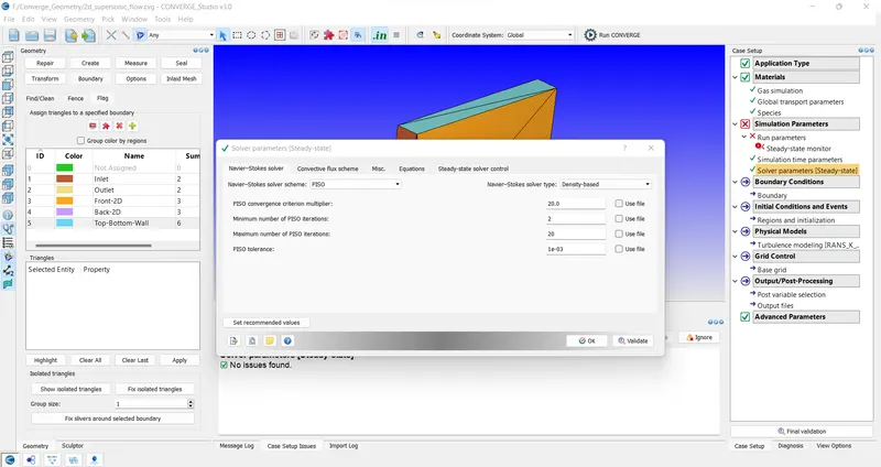
4) In solver parameters select the Navier-stokes solver type as the density-based solver.
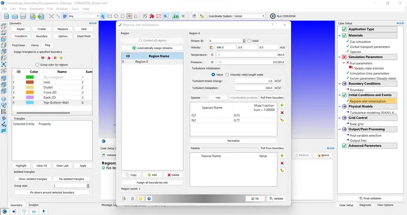
5) Add a new region and include air as species in it. input temperature to be 293K and velocity in the x-direction to be 686m/s.
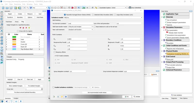
6)In the Physical model select RNG k-ε keeping other values as default.
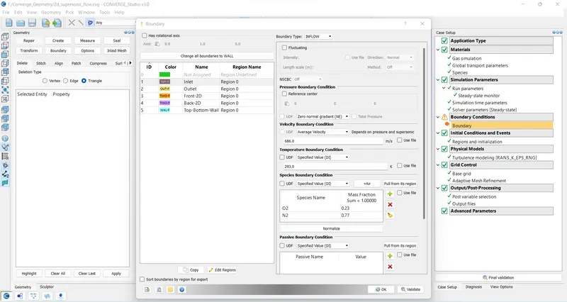
7) For Inlet Pressure: Neuman Boundary condition
Velocity : 646m/s
Temperature: 293K
Outlet Pressure: Neuman Boundary condition
Backflow species: Air
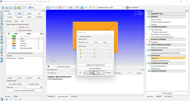
8) Set the base grid to 0.001m for dx, dy, and dz. and check on adaptive mesh refinement.
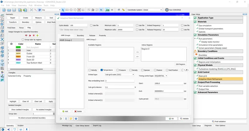
9) In adaptive mesh refinement select embed type as sub-grid scale. Timing control type as Sequential. Max embed leve 2 sub grid criteria 0.001.
9) Do not change anything in Output files and post variable selection. Click on final validation to check for any errors.
Processing input files:
1) Click on file > export > input files
2) Copy and paste licence.lic and mpiexec.exe file in the folder of input files
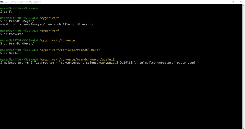
3) Open Cygwin browse to input files folder
4) Enter the following commands
mpiexec.exe -n 6 “C:\Program Files\Convergent_Science\CONVERGE\3.0.16\bin\intelmpi\converge.exe” restricted
5) After completion of the process.
6) Copy and paste the post_convert file in the output folder in the cygwin Enter command
mpiexec.exe -n 6 post_convert
7) Enter the Name for the case selection
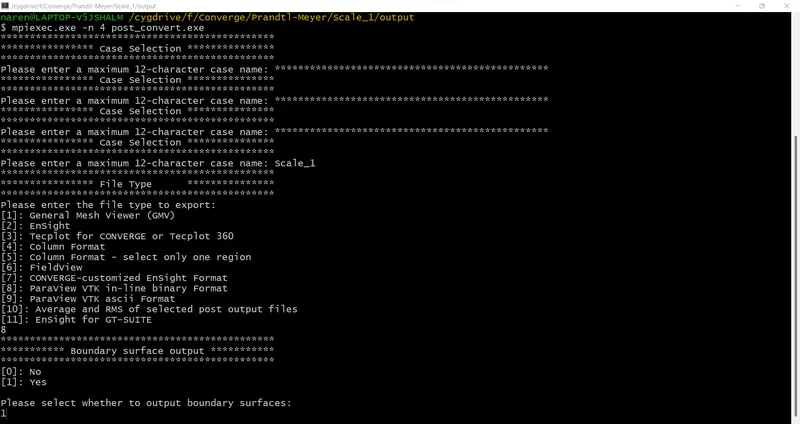
8) Enter file type to export as Paraview VTK in-line binary format
9) Select yes to put boundary surface output
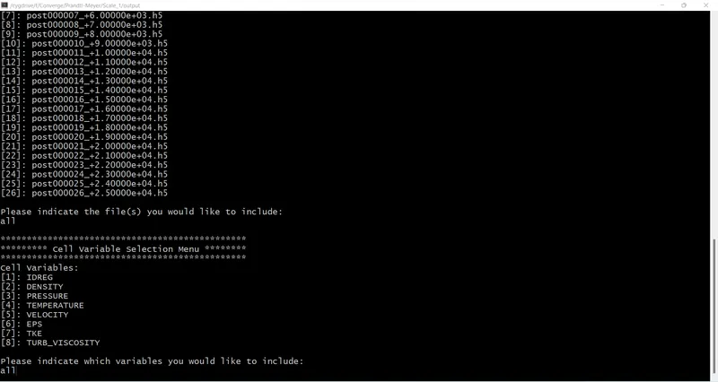
10) Include all file for post processing
11) Include all cell variables
Post-processing of files:
1) Open Paraview for post-processing and open a folder named output and open the file with extension .vtm and click apply.
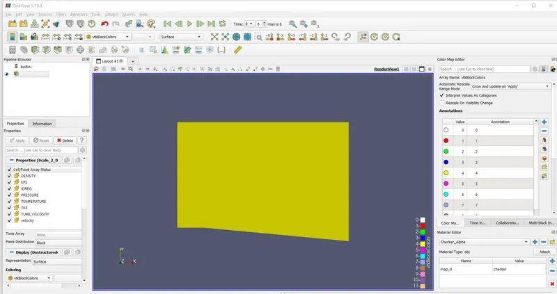
2) Click on slice and along Z normal uncheck triangulate slice and show plane.
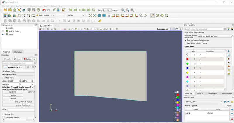
3)Select velocity click play and check on visibility change.
Results:
Sub-Grid scale-0.001
Mesh:https://youtu.be/KKE_cjW5n2o
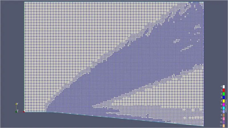
Temperature:https://youtu.be/UNlVSvHdw8U
Velocity:https://youtu.be/EDEZtf6bfYc
Pressure:https://youtu.be/cq32dV6xBPE
Total cell count vs Cycles:
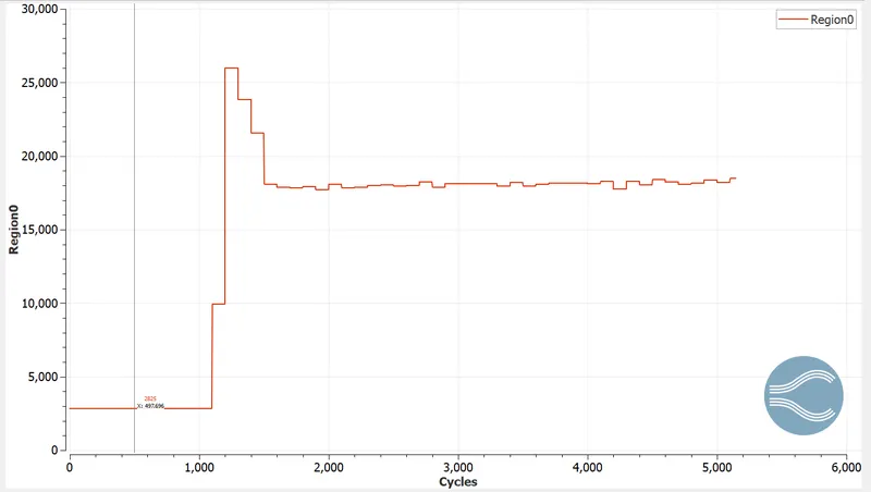
Total cell count ranges from 2825-25986 After 1000 cycles as the AMR starts cell count also increases.
Sub-Grid scale-0.01m
Mesh:https://youtu.be/qoNa0fP47bQ
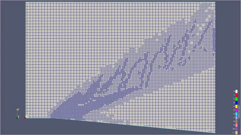
Temperature:https://youtu.be/zPFgeb5o9_o
Velocity:https://youtu.be/2nfp5vJy7NQ
Pressure:https://youtu.be/rvET9EwK6oA
Total cell count vs Cycles:
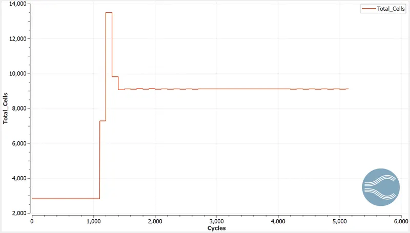
Total cell count ranges from 2825-13896. After 1000 cycles as the AMR starts cell count also increases.
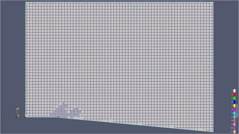
Sub-Grid scale-0.1m
Mesh:https://youtu.be/XrgWupaCzMs
Temperature:https://youtu.be/8Eem4XSHpHA
Velocity:https://youtu.be/ogqkxgLqGhw
Pressure:https://youtu.be/FGCCCcOqvcg
Total cell count vs Cycles:
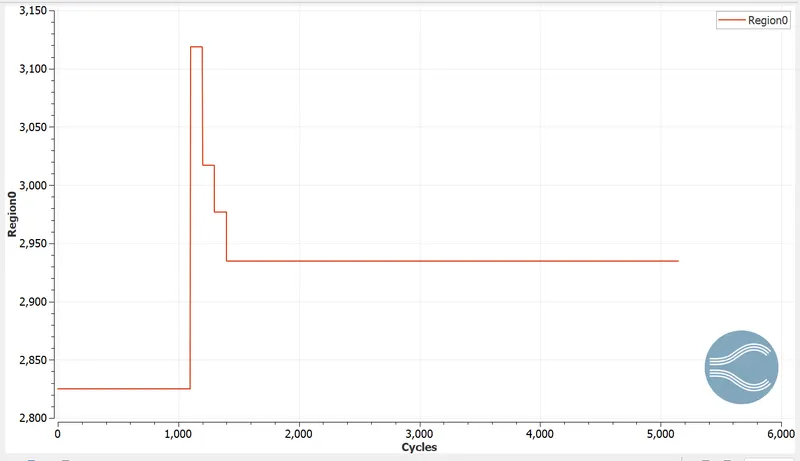
Total cell count ranges from 2825-3119. After 1000 cycles as the AMR starts cell count also increases.