Week 7: Shock tube simulation project
Shock Tube Simulation Using Converge CFD
Aim: Setting up the shock tube problem and simulating Shock flow using Converge CFD.
Objectives:
- Setup a transient shock tube simulation
- Plot the pressure and temperature history in the entire domain - Explain the result
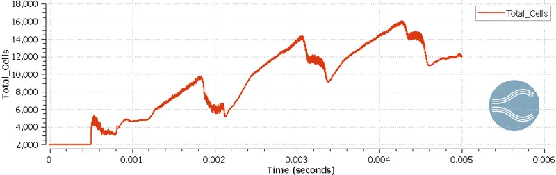
- Plot the cell count as a function of time - Explain the result
Shock Wave:
Shock is an abrupt discontinuity in the flow field and it occurs inflows when the local flow speed exceeds the local sound speed. More specifically, it is a flow whose Mach number exceeds 1.
A shock wave is a type of propagating disturbance that moves faster than the local speed of sound in the medium. Like an ordinary wave, a shock wave carries energy and can propagate through a medium but is characterized by an abrupt, nearly discontinuous, change in pressure, temperature, and density of the medium.
When an object is moving in a flow field the object sends out disturbances that propagate at the speed of sound and adjusts the remaining flow field accordingly. However, if the object itself happens to travel at speed greater than sound, then the disturbances created by the object would not have traveled and communicated to the rest of the flow field and this results in an abrupt change of property, which is termed as a shock in gas dynamics terminology.
Flow simulation in CONVERGE done in 3 steps:
- Geometry preparation and Case setup :
- We use Converge GUI(Graphical User Interface) to set up the case and export input files.
- Solving the problem using input files:
- These input files are solved by Converge in the Terminal (Command-line interface). We USed Cygwin for the command line terminal.
- Post-processing results:
- We convert our solution into Paraview binary format to post-process the results in Paraview
Geometry preparation in CONVERGE CFD:
- Geometry preparation:
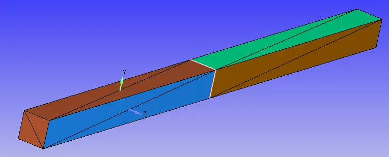
- Import the ".STL" file of the shock tube problem.
- Import the ".STL" file of the shock tube problem.
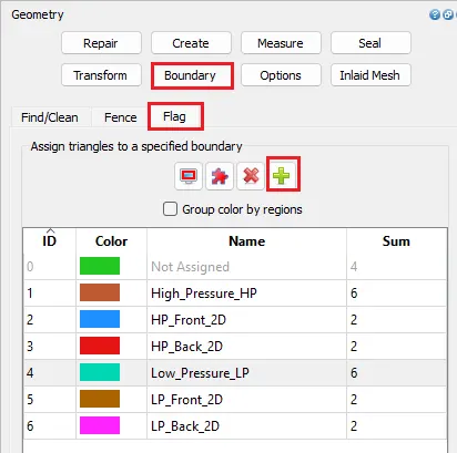
- Boundary setting:
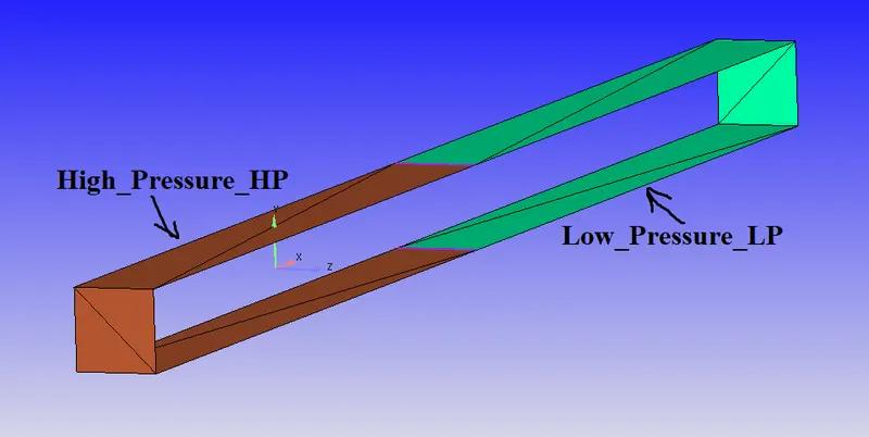
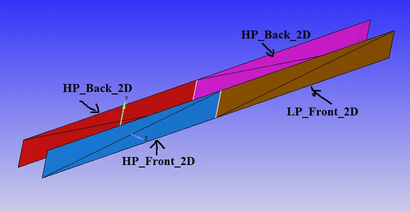
- Create boundary fences were ever required for proper section of triangles.
- By default In CONVERGE, all the surfaces are made up of triangles we have to select respective triangle faces for the boundary.
- Boundaries for the above-created geometry.: High_Pressure_HP, HP_Front_2D, HP_Back_2D, Low_Pressure_LP, LP_Front_2D, LP_Back_2D
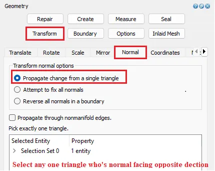
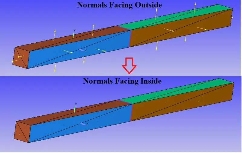
- Normal Transformation:
- All the face normal directions should be facing towards the flow region.
- In this fluid is flowing through the channel but normals are facing outwards. We have to transform the normal's direction.
- Diagnosis:
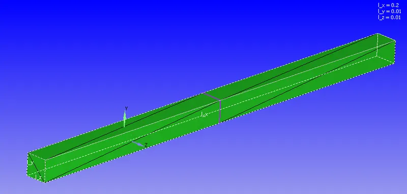
- Checking for any interactions, open edges, Non manifold Problems etc.
Case Setup in CONVERGE CFD:
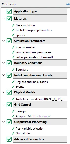
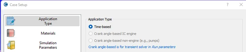
- Application Type :
- Initial Conditions and Events:
- Regions and initialization:
- Adding High pressure and Low-pressure regions in the regions section & initialize them.
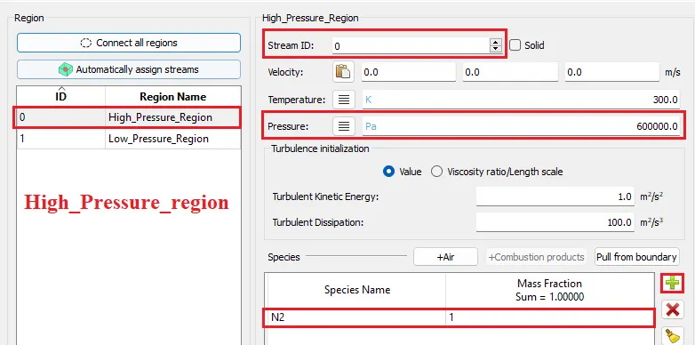
- High_Pressure_Region:
- Steam Id = 0 ;
- Initialization :- Temperature = 300 K ; Pressure = 600000 Pa
- Add N2 species.
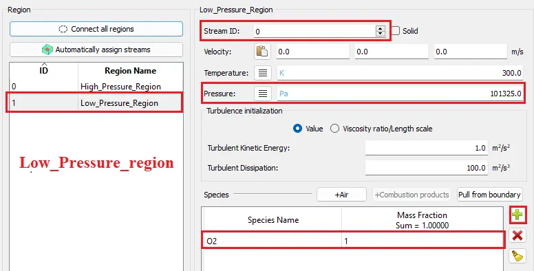
- Low_Pressure_Region:
- Steam Id = 0 ;
- Initialization :- Temperature = 300 K ; Pressure = 101325 Pa
- Add O2 species.
- Events:
- Events are nothing but creating connection and disconnection between two regions for a particular period of time.
- In this simulation, we have created High pressure and low-pressure regions and Initialized them with 600000 Pa and 101325 Pa.
- Initially, we don't want the fluid to flow from the High-pressure region to the Low-pressure region, after some time we have to enable the flow this sudden connection is just like popping a diaphragm in experiments. This sudden expansion creates Shock waves.
- In the simulation, we can't pop a diaphragm this can be achieved by creating Events
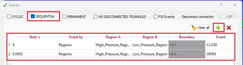
- At 0 seconds High pressure and low-pressure regions are disconnected ==>> Closed ==>> No Flow Takes Place.
- From 0.0005 Seconds High pressure and low-pressure regions are connected ==>> Open ==>> Flow Takes Place.
- Events are nothing but creating connection and disconnection between two regions for a particular period of time.
- Boundary conditions:
- Defining boundary type and conditions:
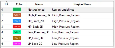
-
Boundary Name Type Boundary Condition
High_Pressure_HP WALL Slip HP_Front_2D Two_D HP_Back_2D Two_D Low_Pressure_LP WALL Slip LP_Front_2D Two_D LP_Back_2D Two_D
- Regions and initialization:
- Simulation Parameters:
- Run Parameters:
- Selecting the Solver & solver type. informing additional things to solve (Energy & Momentum equations).
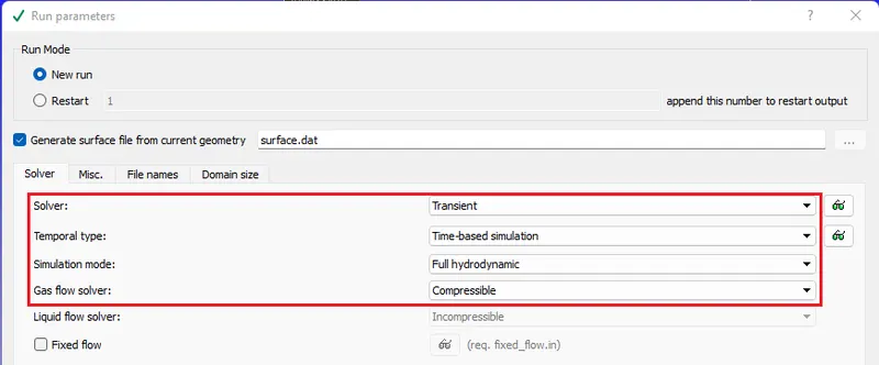
- Simulation Parameter:
- defining star, end time, Minimum & Maximum Timestep sizes.
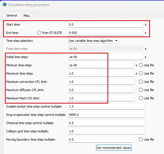
- Solver Parameters:
- Solver Scheme to PISO and Density-based solver.
- under Equations window set precondition to None for all the variables.
- Navier-Stokes Solver Scheme: PISO
- Navier-Stokes solver type = Density-Based.
- Run Parameters:
- Grid Control:
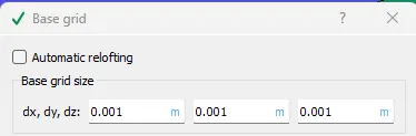
- This is the section where we define meshing size(Grid size).
- Case 1 : dx = 0.001 m, dy = 0.001 m, dz = 0.001 m
- Case 1 : dx = 0.001 m, dy = 0.001 m, dz = 0.001 m
- Adaptive Mesh refinement (AMR):
- In Adaptive Mesh refinement mesh gets auto-refined according to the condition given.
- here we are specifying the maximum number of cells that can be reached after refinement is 200,000 cells.
- firstly we have to shift the Volumetric_region in available regions to active regions.
- For this case, we are using Species-based AMR so that we can monitor the curvature of Species Massfraction. whenever the curvature of the Species Massfraction is greater than the particular value we refine the mesh.
- Embed type: Sub-grid Scale (SGS)
- we have to enter magnitude for sub-grid criterion. for example, if we enter Sub-grid criterion = 0.001 mesh gets auto refined in the region where the Species Massfraction difference between `N` cell and `N-1` cell is greater than the criteria.
- Max embedding level is used to calculate and refine the mesh to the maximum possible limit(minimum size).
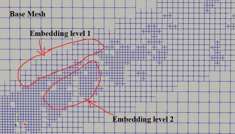
- `text(Grid size) = text(Base grid size)/2^text(Embed level)`
- For this simulation, we used base grid size = 0.8m and embed level = 2
- `text(Smallest possible cell size) =0.001/2^3 = 0.000125 meters`
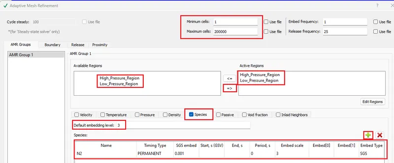
- This is the section where we define meshing size(Grid size).
- Physical Models:
- Turbulence Modelling:
- using Renolds Average Navier stroke equation
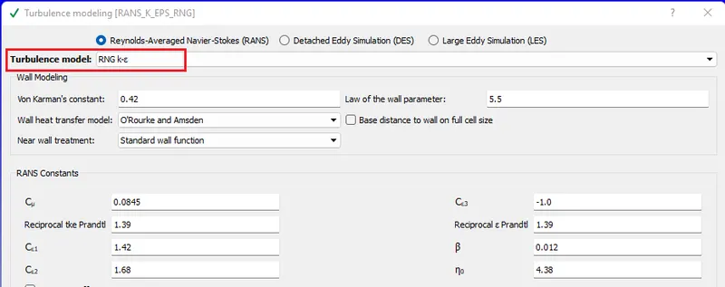
- Turbulence Modelling:
- Output/Post-Processing
- Post Variable selection: select the variables to be monitored for post-processing.
-
S.No Typical variables Geometry/Location 1 Density Region ID 2 Pressure 3 Temperature 4 Velocity 5 Mesh Quality 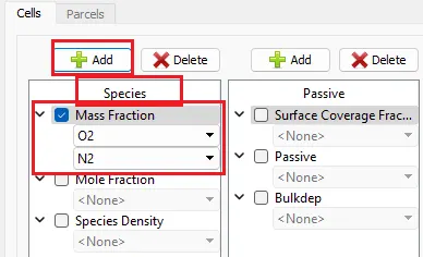
-
S.No Turbulence 1 Dissipation Rate of tke (eps) 2 Turbulent Kinetic Energy(tke) 3 Turbulent Viscosity
-
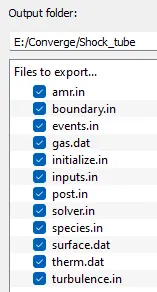
- Exporting Input files:
- Export the input files
- Export the input files
- Post Variable selection: select the variables to be monitored for post-processing.
Solving Channel Flow in Cygwin:
- Go to the directory where input files are exported
- Make mpiexec.exe & converge.exe files globally available.
- "mpiexec.exe -n 4 converge.exe restricted </dev/null> logfile &"
- Use above mentioned line to start calculation in the background
- mpiexec.exe & converge.exe are executable applications to solve the problem
- -n 4:- number of processors
- restricted:- my license is a restricted one.
- </dev/null> logfile:- creates temporary memory to save data with name as logfile at a particular iteration
- & :- To run Calculation in Background
- "tail -10 logfile" command is used to view the last 10 lines of the log file.
- "mpiexec.exe -n 1 post_convert_30_serial_64" command used to convert output files to paraview binary format, so that they can be processed in the paraview.
Post Processing and Results from Paraview:-
- open "..vtm" group file in paraview. This group contains all the solution files.
- use the slice tool to create a contour section plane and plot the contours
Results:
- Mesh:
- T = 0 sec
- T = 0.005 sec
- T = 0 sec
- Mass Fraction N2:
-
- Mass Fraction O2:
- Temperature Profile:
- Velocity Profile:
- Pressure Profile:







Plots:
- Cell Count:
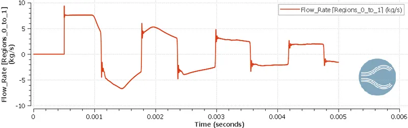
- Flowrate:
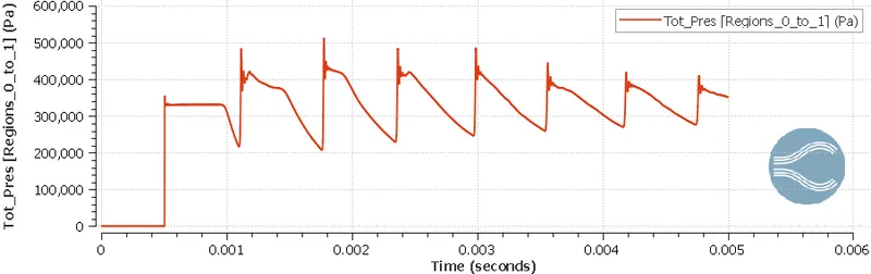
- Pressure:
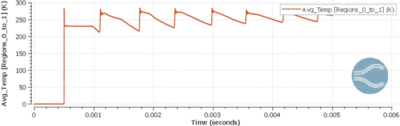
- Temperature:
- Velocity:
Conclusions:
- Till the 0 to 0.0005 seconds high-pressure regions and low-pressure regions are closed and disconnected from each other. When the simulation reaches 0.0005 seconds Even called OPEN opens the connection between two regions this sudden expansion from 6 bar to 1 Atm pressure produces sudden shock into the low-pressure region leading to an increase in temperature of the system and velocity of the particles increases. From the animations, we can see how temperature, velocity are varying. When the expansion reaches the boundary it reflects fack and creates oscillations continuously till the system reaches to steady-state.
- We used adaptive mesh refinement with Subgrid criteria of 0.001. For this simulation, mesh gets auto-refined in the zone where the Species Massfraction difference between the `N` cell and `N-1` cell is greater than the criteria 0.001. from the Mesh Contours we can visualize the Mesh refined zones.