Week 7 - Mini project - Flow over an Airfoil

AIM

1. To compare the results obtained at a particular angle of attack using different turbulence models with experimental data and choose the better turbulence model to solve the problem for the remaining angle of attacks.
2. To simulate the flow over NACA 2412 airfoil and find the coefficient of lift and drag at different angles of attack.

THEORY

An airfoil is the cross-sectional shape of a wing, blade (of a propeller, rotor, or turbine), or sail (as seen in cross-section).

The lift on an airfoil is primarily the result of its AOA. When oriented at a suitable angle, the airfoil deflects the oncoming air (for fixed-wing aircraft, a downward force), resulting in a force on the airfoil in the direction opposite to the deflection. This force is known as aerodynamic force and can be resolved into two components: lift and drag. Most foil shapes require a positive angle of attack to generate lift, but Cambered airfoils can generate lift at zero angle of attack. This "turning" of the air in the vicinity of the airfoil creates curved streamlines, resulting in lower pressure on one side and higher pressure on the other. This pressure difference is accompanied by a velocity difference, via Bernoulli's principle, so the resulting flow field about the airfoil has a higher average velocity on the upper surface than on the lower surface.

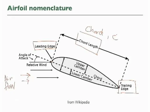
Airfoil nomenclature:

1. Mean camber line- A line drawn halfway between the upper and lower surfaces of the aerofoil.
2. Leading-edge- It is the front edge of aerofoil where maximum curvature can be found.
3. Trailing edge- It is the rearmost edge of an aerofoil.
4. Chord line- It is the connecting line between leading and trailing edge and it is straight.
5. Chord length- It is the length of the chord line.
6. Camber- It is the maximum perpendicular distance between the mean camber line to chord line.
7. Thickness- It is measured either perpendicular to the camber line or perpendicular to the chord line.
8. The angle of attack- It is defined as the angle between the chord line and the relative wind or flight path.

Geometry Creation

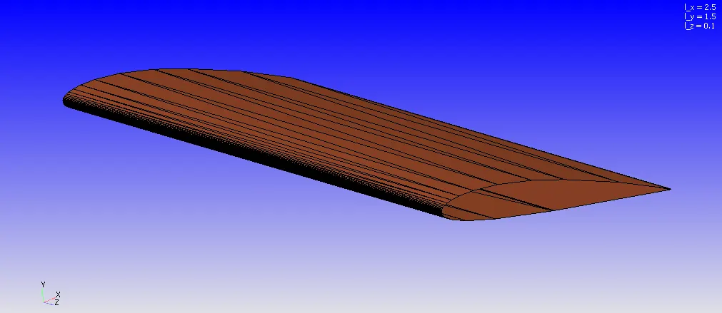
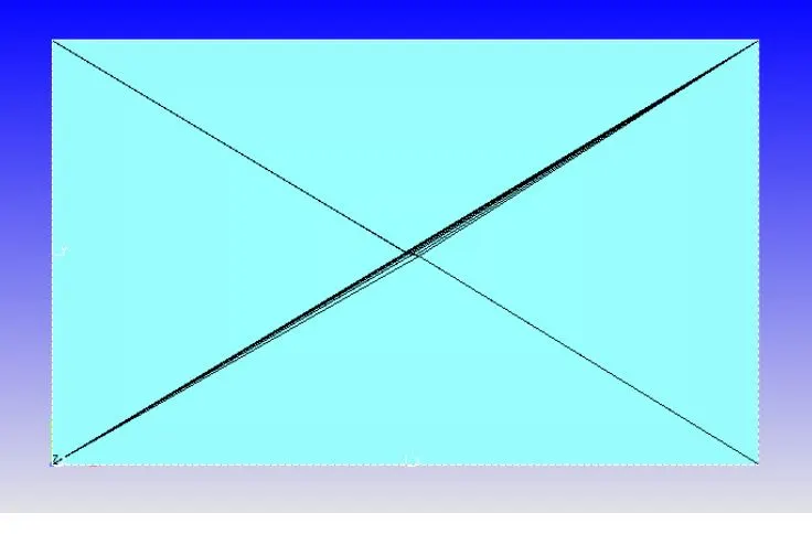
The NACA 2412 coordinate points for chord length 0.1m were imported from airfoiltools.com into CATIA (a CAD software), and the required airfoil was generated by joining these coordinate points using the spline tool. This airfoil geometry is enclosed by a box (virtual wind tunnel) and is saved in STL format. The different angles of attack can be obtained by using the rotate tool. Once the geometry is saved in STL format, it can be imported into Converge CFD and simulations performed.

http://airfoiltools.com/airfoil/naca4digit

Velocity Calculation

Re=

Re=200000

Density=1.225 kg/m^3

l = 0.1 ,

v=30.14 m/s

CASE SETUP
1. Parameters:

Solver= transient

Temporal type= time-based simulation

Simulation mode= full-hydrodynamic

Gas flow solver= compressible

2. Simulation time parameters:

Start time= 0s

End time= 1s

Initial time-step= 1e-5s

Minimum time-step= 1e-5s

Maximum time-step= 1s

Maximum convection CFL limit= 1

3. Regions and initialization:

Stream ID= 0

Velocity(x,y,z)= (30.14, 0, 0)

Temperature= 300K

Pressure= 101325Pa

Species= air

4. Boundary:

Inlet:

Inflow boundary condition

Velocity(x,y,z)= (30.14, 0, 0)

Temperature= 300K

Species= air

Outlet:

Outflow boundary condition

Pressure= 101325Pa

Species backflow= air

Front2D, Back2D:

2D boundary condition

Top_bottom_wall:

Slip wall boundary condition

Wall motion= stationary

Surface moement= fixed

Airfoil_wall:

No-slip wall boundary condition

Wall motion= stationary

Surface moement= fixed

5. Turbulence model used:

Part1: RNG K-epsilon, K-omega SST turbulence model

Part2: K-omega SST turbulence model

6. Base grid:

Base grid size (x, y, z)= (0.02, 0.02, 0.2)m

Fixed ebedding

Entity type= boundary

Boundary ID= airfoil_wall

Mode= sequential

Scale= 2

Embed layers= 10

Start time= 0s

End time= 10s

7. Output files:

Wall output= boundaries only

Time interval for writing 3D output data files= 0.01s.

Time interval for writing text output= 1e-5s

Time interval for writing restarting output= 0.01s

Maximum number of restarting files saved= 3

RESULT

Case 1

Angle of attack=1°

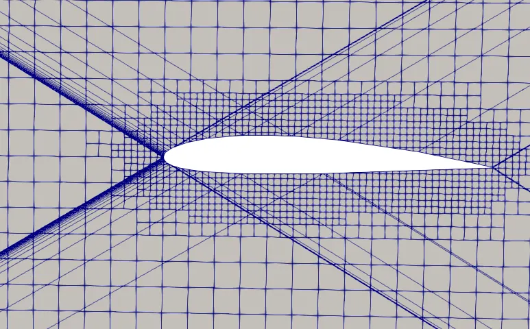
Mesh

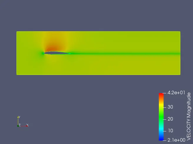
Velocity Contour

PLOT

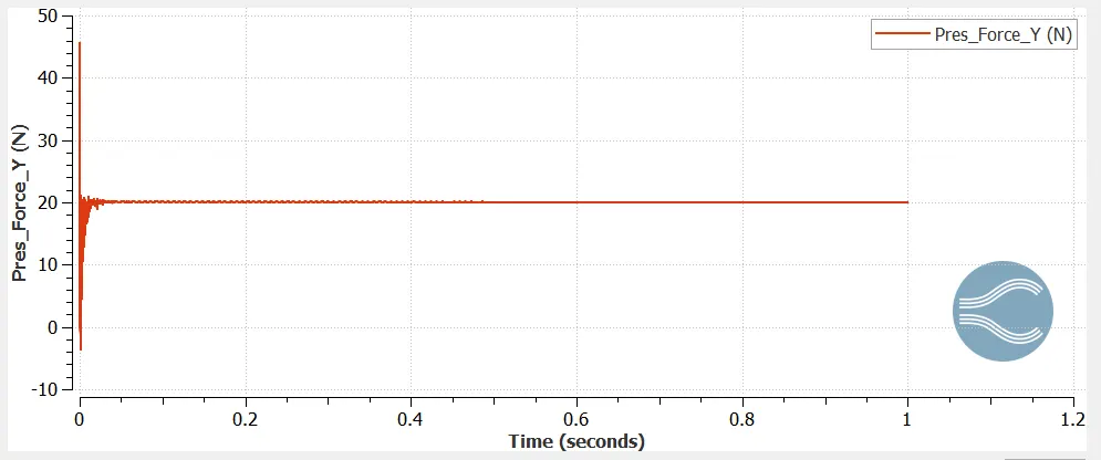
Pressure force on Y direction is nothing but Lift force(L)

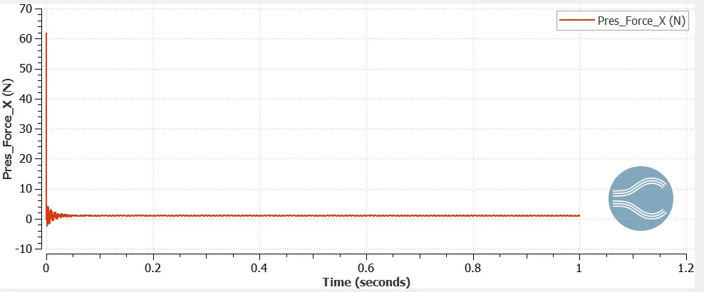
Pressure force on X direction is nothing but Drag force(D)

from Above graphs

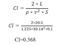
L=20.5N

D=1.5N

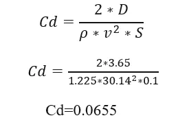
Calculation of Coefficient of drag(Cd)

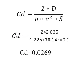
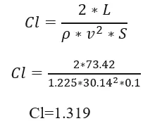
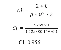
Calculation of Coefficient of lift(Cl)

Case 2

Angle of attack=5°

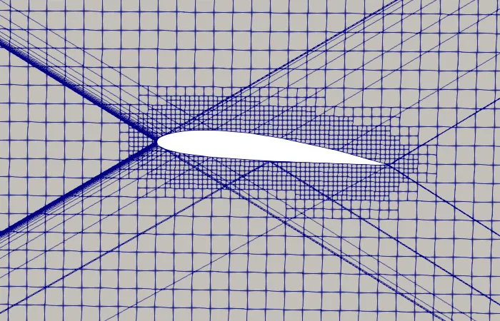
Mesh

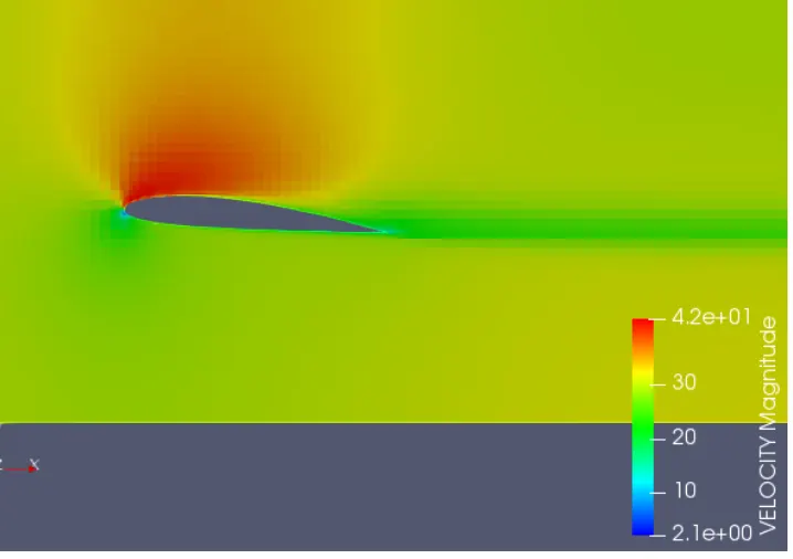
Velocity Contour

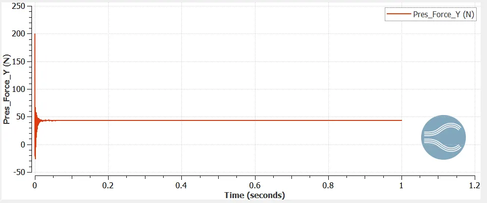
Pressure force on Y direction is nothing but Lift force(L)

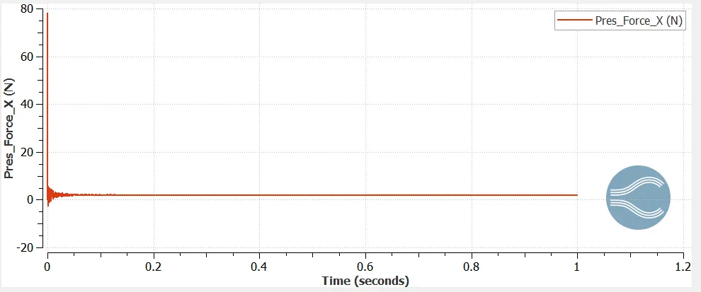
Pressure force on X direction is nothing but Drag force(D)

from Above graphs

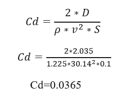
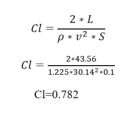
L=43.56N

D=2.035N

Calculation of Coefficient of drag(Cd)

Calculation of Coefficient of lift(Cl)

Case 3

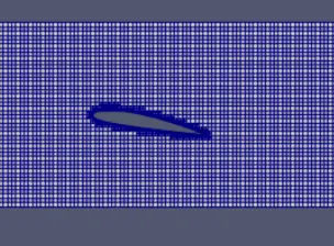
Angle of attack=10°

Mesh

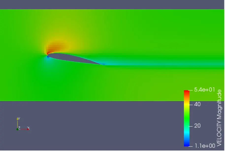
Velocity Contour

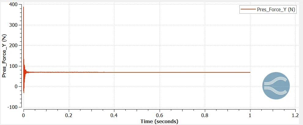
Pressure force on Y direction is nothing but Lift force(L)

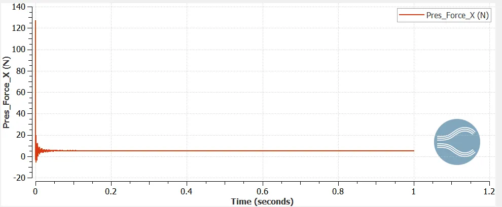
Pressure force on X direction is nothing but Drag force(D)

from Above graphs

L=73.42N

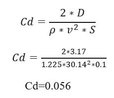
D=3.17N

Calculation of Coefficient of drag(Cd)

Calculation of Coefficient of lift(Cl)

Case 4

Angle of attack=15°

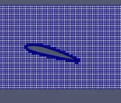
Mesh

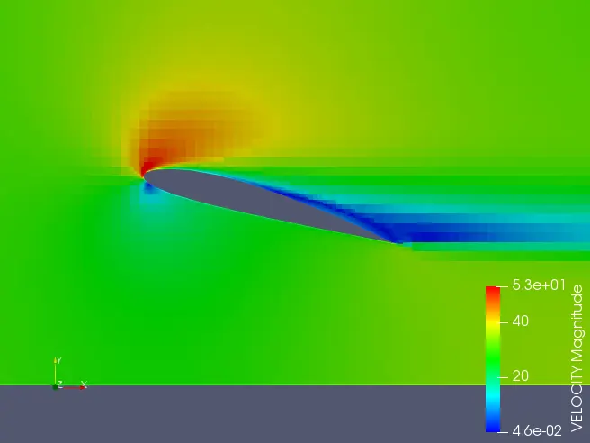
Velocity Contour

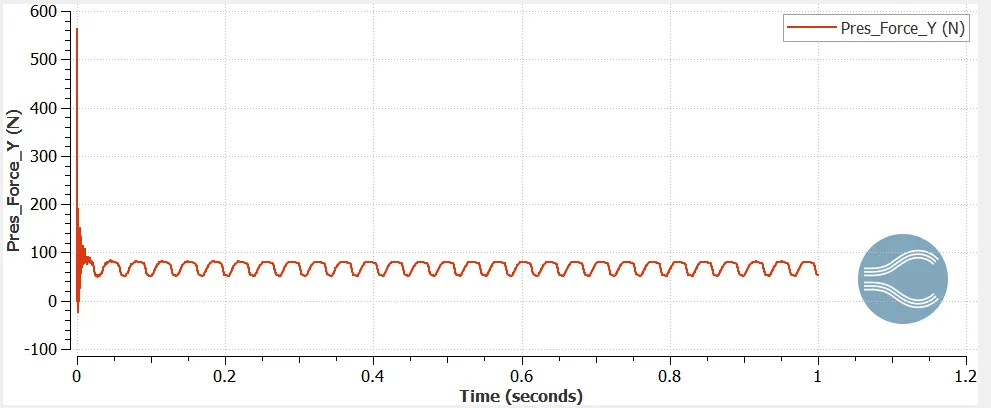
Pressure force on Y direction is nothing but Lift force(L)

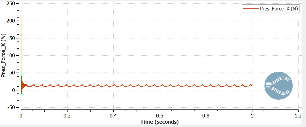
Pressure force on X direction is nothing but Drag force(D)

from Above graphs

L=53.28N

D=3.65N

Calculation of Coefficient of drag(Cd)

Calculation of Coefficient of lift(Cl)

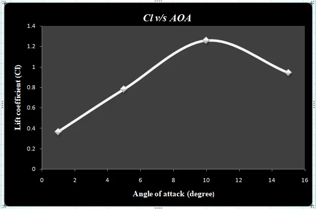
AOA	Cd	Cl
1°	0.0269	0.368
5°	0.0365	0.782
10°	0.056	1.319
15°	0.065	0.956

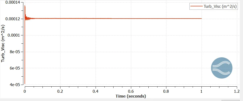
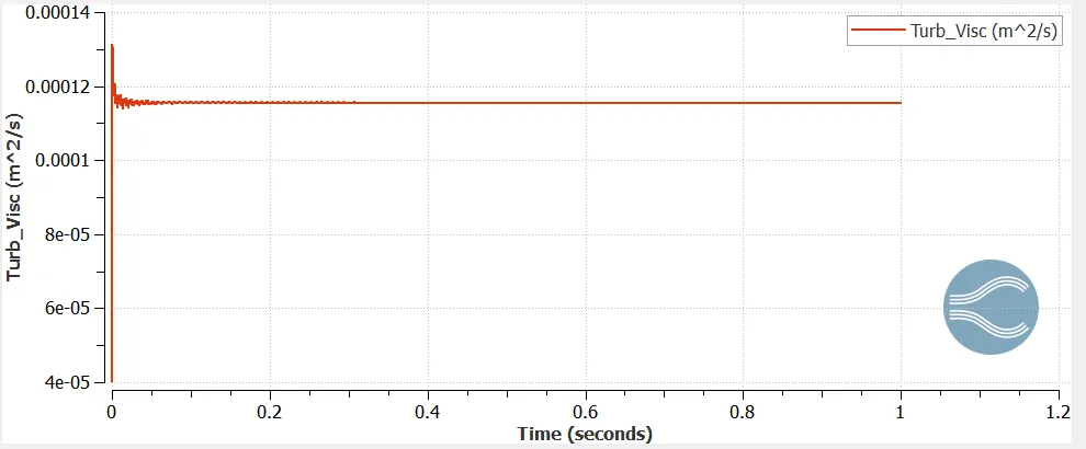
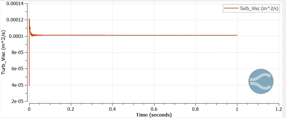
EFFECT OF TURBULENCE (TURBULENT VISCOSITY) ON DIFFERENT AOA

1°

5°

10°

15°

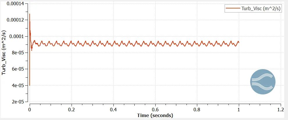
With the increase in AOA the turbulent viscosity decreases, this means that the flow over an airfoil is slowly separating due to the growth of boundary layer and formation of vortices.

AOA vs Cl

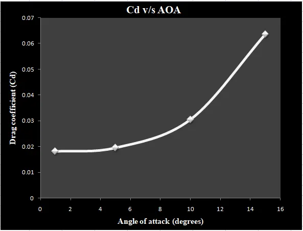
AOA vs Cd

CONCLUSION

*The drag force and coefficient of drag increases with the increase in the angle of attack of the airfoil due to the increase in the frontal area.

*The accuracy of the solution obtained can be improved by reducing the mesh grid size, increasing the embed scaling, and by maintaining the value of yplus term within a certain limit for the given turbulence model.

*The flow is attatched to the body and the lift generation increases till the effect of stallling comes into picture. Once stalling happens the lift generation

decreases and flow seperation takes place leading to the formation of vortices and eddies at the trailing edge.