Channel flow simulation using CONVERGE CFD
AIM:
To simulate channel flow using converge with three different given mesh size.
Case-1: Grid size- dx=3e-3 m, dy=3e-3 m, dz=3e-3 m
Case-2: Grid size- dx=2.5e-3 m, dy=2.5e-3 m, dz=2.5e-3 m
Case-3: Grid size- dx=2e-3 m, dy=2e-3 m, dz=2e-3 m
DESCRIPTION:
Channel flow is a very basic problem of CFD. In this challenge, the a channel is constructed and a steady state simulation is run for three different mesh sizes and the results are compared. The steady state solver is set up by monitoring the velocity obtained at the output. A sample of 100 output is taken and checked for variation. If the variation is within tolerance, then the simulation is stopped. Even though the total running time for the simulation is specified, the steady state solver stops once the variation is within tolerance and thereby saving a lot of time and money in the process
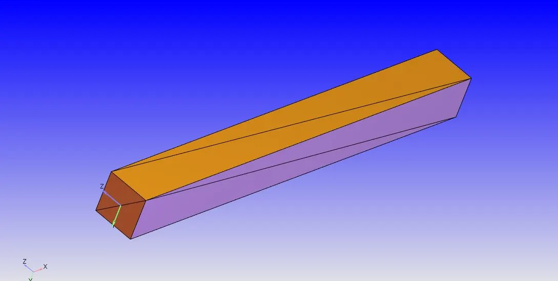
1.Geometry
Centre = (0.05,0,0)
Size=(0.1,0.01,0.01)
2.Boundary Creation
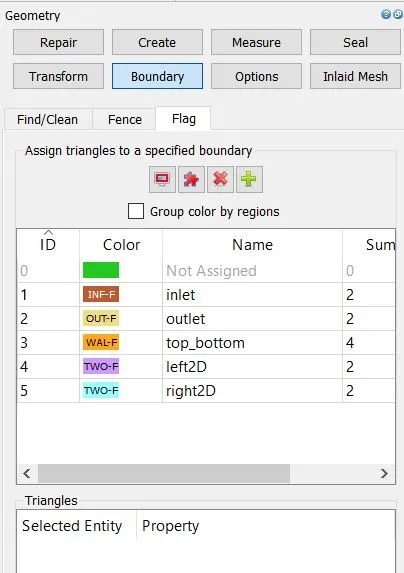
After creating the box Geometry, The Boundary tag was created along with different boundary id and colouring. A total of 5 different boundaries tag was created for 6 different faces of the box with each face split into two triangles. To create the boundaries naming, the "Boundary" command in the "Geometry" dock was used, and then the faces were appointed to appropriate tags along with id.
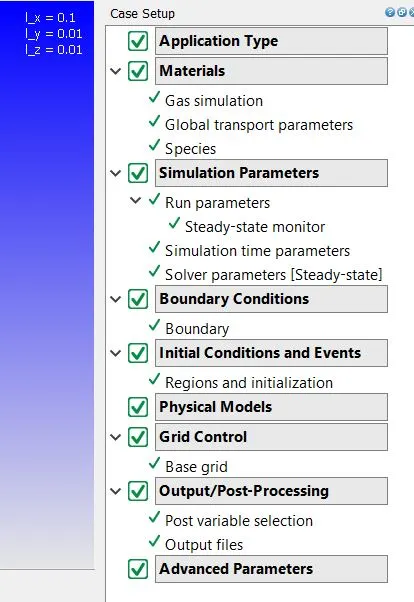
2.Case Setup
Applications- Time based
Materials - Air
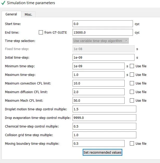
Simulation Parameters:
Boundary conditions
|
Boundary_Name |
Boundary_Type |
Paramter_Defined |
Boundary ID |
|
1.Inlet |
Inflow |
100001 Pa |
1 |
|
2.Outlet |
OutFlow |
100000 Pa |
2 |
|
3.Top-Bottom-walls |
Wall |
Specified Value(300k) No-Slip Condition |
3 |
|
4.Front2d |
Two_D |
4 |
|
|
5.Back2d |
Two_D |
5 |
Regions & Initialization:
Species:- O2 (0.77) & N2 (0.23)
Pressure :100001Pa
Temperature:300K
CASE 1
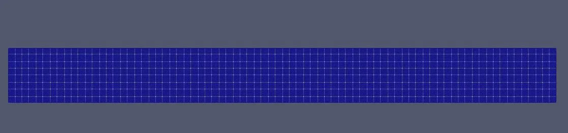
Mesh size
dx = 2e-4m, dy = 2e-4m, dz = 2e-4m
Velocity Contour
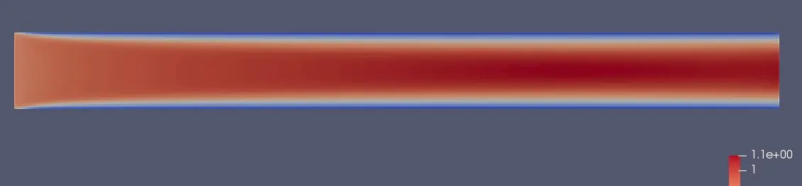
Pressure Contour

CASE 2:
Mesh size
- dx = 1.5e-4m, dy = 1.5e-4m, dz = 1.5e-4
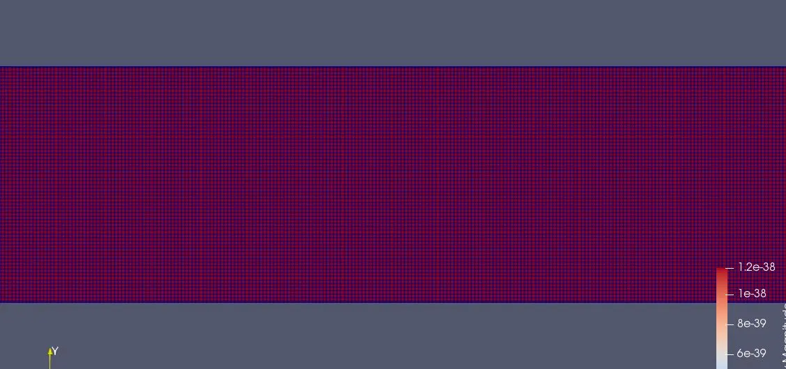
Velocity Contour

Pressure Contour
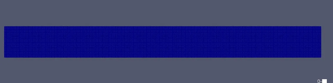
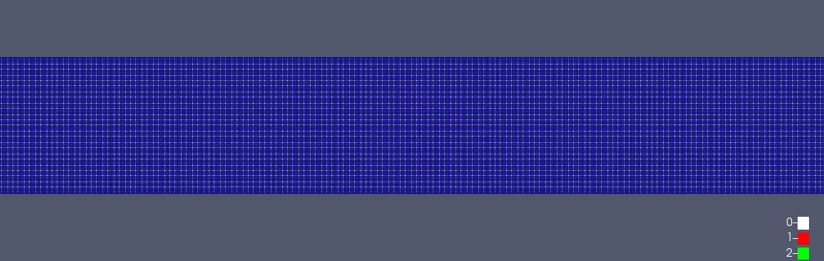
CASE 3
Mesh size
dx = 1.2e-4m, dy = 1.2e-4m, dz = 1.2e-4m
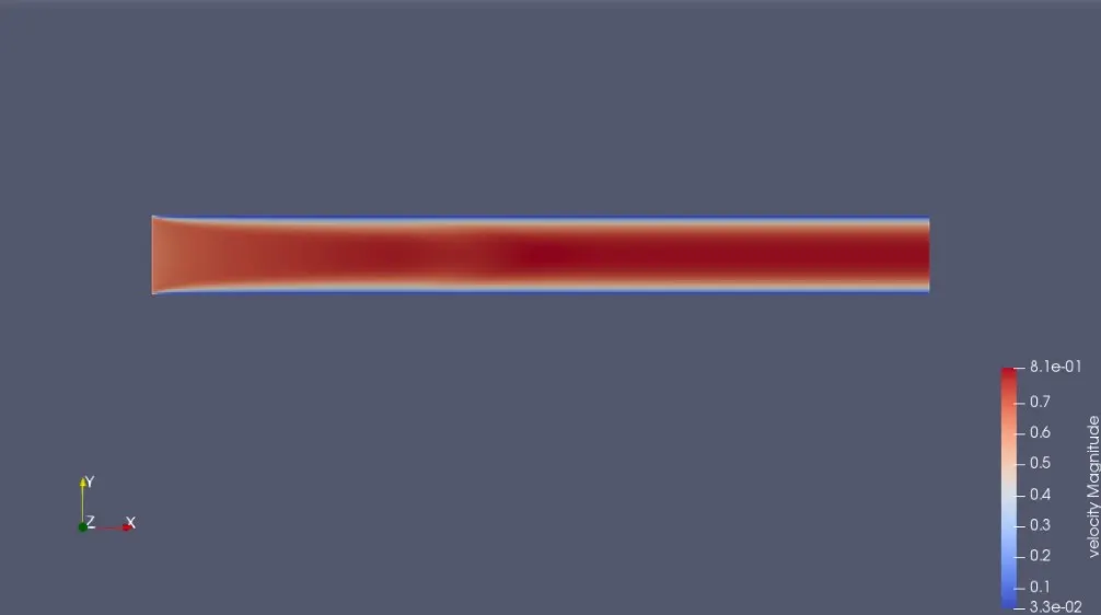
Velocity Contour
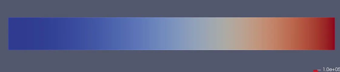
Pressure Contour
RESULT
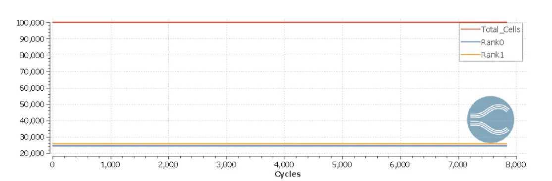
Total cell count plot
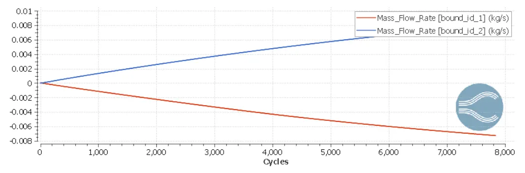
Mass flow rate plot at inlet and outlet
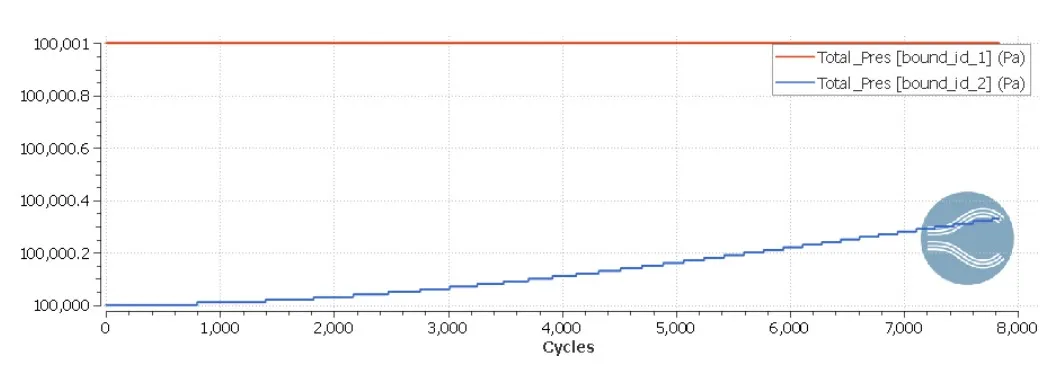
Pressure plot at inlet and outlet
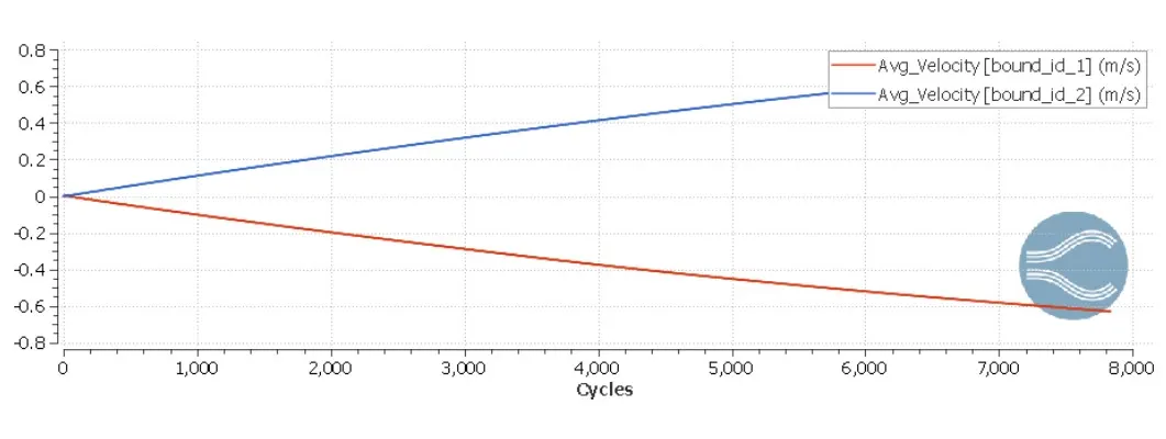
Average Velocity plot at Inlet And Outlet
The Youtube link for the animation of velocity and pressure contours for the grid size of (2.0e-4) are given below
The Youtube link for the animation of velocity and pressure contours for the grid size of (1.5e-4) are given below
The Youtube link for the animation of velocity and pressure contours for the grid size of (1.2e-4) are given below
Conclusion
1.The velocity is high at the centre of the wall because of no slip condition.
2.As we reduce the number of element the simulation time is also reduced.
- From velocity plots we can observe that initially velocity is high and moves smoothly for some cycles and finally becoming stable.Initially we can observe that there are more oscillations which goes on becoming smaller with number of cycles, it reaches to a point of convergence after some cycles.
- The mass flow rate profiles for both inlet and outlet is same as the mass (air) is same at both inlet and outlet. Initially we can observe that there are more oscillations which goes on becoming smaller with number of cycles, it reaches to a point of convergence after some cycles.
- From cell contour we can observe that as the base grid is being decreased the total cell count is being increased.
- In pressure plots one curve indicates total pressure at inlet and the other indiactes the total pressure at outlet boundary. Initially there are some fluctuations but after some some cycles it remained constant.