Week 7: Literature review - RANS derivation and analysis

RANS Derivation and Analysis

Aim:

1. To apply the Reynolds Decomposition to the Navier-Stokes Equation and derive the Reynolds Averaged Navier Stokes Equation.
2. To explain the term Reynolds Stress.
3. To explain about the Molecular and Turbulent Viscosity and their Difference.

Navier - Stokes Equation:

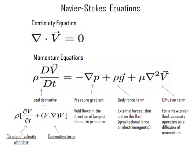
Navier-Stokes equation or NSE is a set of equations which can be able to predict the velocity, pressure or the characteristics of the flow of the fluid at each and every point. The eqn. are:

Continuity eqn.:`grad.vecV =0`

Momentum eqn.: `rhofrac(dvecV)(dt)=-gradp+mugrad^2 vecV +rhovecg`

Continuity Eqn.:

`grad.vecV =0`

This equation simply says that mass is conserved. Here the `vecV` is the velocity u, v, w for all x, y, z three directions. If you take a flow of river, it is impossible for the fluid to disappear at some point. In other words, at some points, the fluid would change only it’s shape, if the fluid converges at a particular point, then `grad.vecV <0` . If the fluid diverges at a particular point, then `grad.vecV >0` . But here at the analyzation of fluid flow that has no source of convergance and divergence, the divergence of the velocity is zero and hence the mass is conserved.

Momentum Equation:

`rhofrac(dvecV)(dt)=-gradp+mugrad^2vecV+rhovecg`

This particular eqn. just arise from Newton’s second law, F = ma which gives us the value of the net force acting on some point of fluid. Due to these forces the velocity, pressure & characteristics of fluid may vary frequently. Mass is `rho`and acceleration is `frac(dvecV)(dt)`which also is the rate of change of velocity. The Internal forces which acts by it’s own fluid molecules which are all pressure forces `(gradp)`and Frictional forces `(mugrad^2vecV)`which causes by friction acting between the fluid molecules and the External forces, which acts due to the external objects and that is F which is a Gravitational force and that is `rhovecg`which acts in all three directions respectively.

Turbulence and Turbulence Modelling:

• In NS equation, the two most dominating terms are Convection term `((V*grad)V)`and the Viscous or Diffusion term `(mugrad^2vecv)`.Here, If the Diffusion term is greater than the Convective term, the resulting flow will be smooth or the flow might be a laminar and if we cancelled out the Convective term from this equation, the entire NS equation can easily be solved. But if the Convective term is greater than Diffusion term, the resulting flow would be Turbulent, which consists of some Eddies. This gives rise to the Turbulence.
• Turbulence occurs in 3 dimensional, random and chaotic and it always will be Fluctuating.
• Due to this, solving the Navier stokes equation is really tough and time consuming by practically and computationally.
• So that, the Turbulence Modelling like RANS, LES and several equations like K-epsilon, K-omega is been introduced in more user-friendly manner by getting required results.
• For Shock flow, conjugate heat transfer problem or to analyze rotary components like turbine, pumps,etc., we would use Turbulence Modelling.

RANS Modelling :

• In order to analyze the fluid flow in boundary layer, the three equations that would govern the flow is Continuity, Momentum and Energy equation for any type of geometry.
• If we simulate a geometry with a fine mesh and apply these 3 equations, it is capable to capture the both the effects of laminar and turbulent flow and can give us the results and this approach is called Direct Numerical Simulation.
• But it is almost impractical with current technology and also would take million hours and huge number of computational mesh with very small time steps and Engineers also don’t need that kind of accurate results, which the quantities will be more fluctuating with respect to the absolutely small time steps, due to which would take more time.
• So the Idea of the Turbulence modelling is to simulate a geometry with coarser mesh over a sufficient larger time step or time scale, which still would capture the turbulent effects and would also gives us the averaged quantity values with an amount of time.
• RANS & LES (Large Eddy Simulation) are the most common methods to simulate and capture the turbulent flow and its effects. Though LES gave us the more effects & flow of turbulent, most of the Engineers would look only for RANS since it gives the sufficient turbulent flow effects which particularly affect our results and gives averaged value of our expected quantity.
• RANS would give sufficient turbulent and eddies effects that incorporate our expected quantity whereas LES (can be used in a failure analysis) gives the unwanted eddy motion and also it is little bit higher cost and time consuming computationally than RANS.

RANS Derivation:

• The approach of RANS is taking the Navier-Stokes equation and applying the Reynolds decomposition in NS equation and then integrating it over a large enough time scale with some assumptions and ending with some unknown terms.
• The reason for integrating over large enough time step or time scale is to capture only the turbulent flow or eddy flow which affect our quantities and to lose the unwanted eddy flows or turbulent effects which nothing to do by capturing them.
• This process is called Reynolds Averaging.

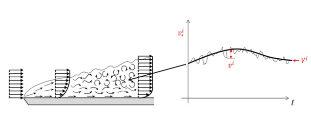
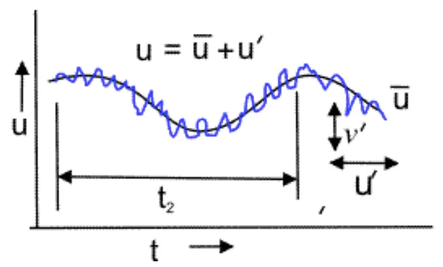
• Reynolds Decomposition: Reynolds decomposition is a mathematical technique used to separate the expectation Mean value of a quantity from its fluctuations.

u(x,y,z,t) = `bar u`(x,y,z) + u′(x,y,z,t)

v(x,y,z,t) = `bar v`(x,y,z)+ v′(x,y,z,t)

w(x,y,z,t) = `bar w`(x,y,z) + w′(x,y,z,t)

• Since, we are time averaging larger than the turbulent time scale (averaging with respect to time), is only a function of space and not a function of time and these time averaged quantities are what engineers do really want.

Time-Averaging formula:

• `bar u(x,y,z)=frac(1)(Deltat)int_t^(t+Deltat)u(x,y,z)dt`
• The time integration of fluctuating component is zero.

`frac(1)(Deltat)int_t^(t+Deltat)u'(x,y,z)dt=0`

Proof:

`u^' (x,y,z,t)=frac(1)(Deltat)int_t^(t+Deltat)u(x,y,z,t)dt-frac(1)(Deltat)int_t^(t+Deltat)bar u(x,y,z)dt`

`=bar u(x,y,z)-bar u(x,y,z)`

`=0`

RANS equation Derivation:

• Applying the Reynolds averaging process to the continuity equation:

`frac(delu)(delx)+frac(delv)(dely)=0`

`frac(del(bar u+u'))(delx)+frac(del(bar v+v'))(dely)=0`

`frac(1)(Deltat)int_t^(t+Deltat)frac(delbar u)(delx)dt+frac(1)(Deltat)int_t^(t+Deltat)frac(delu')(delx)dt+ frac(1)(Deltat)int_t^(t+Deltat)frac(delbar v)(dely)dt+frac(1)(Deltat)int_t^(t+Deltat)frac(delv')(dely)dt=0`

• Cancelling the Fluctuating components and since Time-averaging a mean or averaged velocity has the same value, we get

`frac(delbar u)(delx)frac(1)(Deltat)int_t^(t+Deltat)dt+frac(delbar v)(dely)frac(1)(Deltat)int_t^(t+Deltat)dt=0`

`frac(delbar u)(delx)(frac(t+Deltat-t)(Deltat))+frac(delbar v)(dely)(frac(t+Deltat-t)(Deltat))=0`

`frac(delbar u)(delx)+frac(delbar v)(dely)=0`

• Therefore, the time-averaged continuity eqn. is `grad.barvecv=0`
• Now making the Momentum equation to more convinient form, before applying the Reynolds Averaging Process.

`rho(frac(delu)(delt)+ufrac(delu)(delx)+vfrac(delu)(dely))=-frac(delp)(delx)+mufrac(del^2u)(dely^2)`

`frac(delu)(delt)+ufrac(delu)(delx)+vfrac(delu)(dely)=-frac(1)(rho)frac(delp)(delx)+frac(mu)(rho)frac(del^2u)(dely^2)`

`frac(delu)(delt)+ufrac(delu)(delx)+vfrac(delu)(dely)=-frac(1)(rho)frac(delp)(delx)+nufrac(del^2u)(dely^2)`

where `nu` is Kinematic Viscosity.

• Adding `u(frac(delu)(delx)+frac(delv)(dely))`in L.H.S:

`frac(delu)(delt)+ufrac(delu)(delx)+vfrac(delu)(dely)+u(frac(delu)(delx)+frac(delv)(dely))=-frac(1)(rho)frac(delp)(delx)+nufrac(del^2u)(dely^2)`

`frac(delu)(delt)+ufrac(delu)(delx)+vfrac(delu)(dely)+ufrac(delu)(delx)+ufrac(delv)(dely)=-frac(1)(rho)frac(delp)(delx)+nufrac(del^2u)(dely^2)`

`frac(delu)(delt)+2ufrac(delu)(delx)+vfrac(delu)(dely)+ufrac(delv)(dely)=-frac(1)(rho)frac(delp)(delx)+nufrac(del^2u)(dely^2)`

Substitute `frac(del(uv))(dely)=vfrac(delu)(dely)+ufrac(delv)(dely)`and `2ufrac(delu)(delx)=frac(delu^2)(delx)`, we get

`frac(delu)(delt)+frac(delu^2)(delx)+frac(del(uv))(dely)=-frac(1)(rho)frac(delp)(delx)+nufrac(del^2u)(dely^2)`

Now, applying the Reynolds averaging process,

`frac(1)(Deltat)int_t^(t+Deltat)(frac(del(bar u+u'))(delt)+frac(del(bar u+u')^2)(delx)+frac(del((bar u+u')(bar v+v')))(dely))dt=-frac(1)(rho)frac(1)(Deltat)int_t^(t+Deltat)frac(del(bar p+p'))(delx)dt+nufrac(1)(Deltat)int_t^(t+Deltat)frac(del^2(bar u+u'))(dely^2)dt`

`frac(1)(Deltat)int_t^(t+Deltat)(frac(delbar u)(delt)+frac(delu')(delt)+frac(delbar u^2)(delx)+frac(delu'^2)(delx)+frac(del2bar u u')(delx)+frac(delbar ubar v)(del y)+frac(delbar uv')(dely)+frac(delu'bar v)(dely)+frac(delu'v')(dely))dt=-frac(1)(rho)(frac(1)(Deltat)int_t^(t+Deltat)frac(delbar p)(delx)dt+frac(1)(Deltat)int_t^(t+Deltat)frac(delp')(delx)dt)+nu(frac(1)(Deltat)int_t^(t+Deltat)frac(del^2bar u)(dely^2)dt+frac(1)(Deltat)int_t^(t+Deltat)frac(delu'^2)(delx)dt)`

`frac(delbar u)(delt)+frac(delbar u^2)(delx)+frac(1)(Deltat)int_t^(t+Deltat)frac(delu'^2)(delx)dt+frac(delbarubarv)(dely)+frac(1)(Deltat)int_t^(t+Deltat)frac(delu'v')(dely)=-frac(1)(rho)frac(delbarp)(delx)+nufrac(del^2baru)(dely^2)`

`frac(delbaru)(delt)+frac(delbar u^2)(delx)+frac(delbarubarv)(dely)=-frac(1)(rho)frac(delbarp)(delx)+nufrac(del^2baru)(dely^2)-frac(1)(Deltat)int_t^(t+Deltat)frac(delu'^2)(delx)dt-frac(1)(Deltat)int_t^(t+Deltat)frac(delu'v')(dely)dt`

• So, we get as usual form of Navier-Stokes equation, only the averaging has been done, except the two terms `frac(1)(Deltat)int_t^(t+Deltat)frac(delu'^2)(delx)dt` and `frac(1)(Deltat)int_t^(t+Deltat)frac(delu'v')(dely)dt`.
• From the above equation, the term `frac(1)(Deltat)int_t^(t+Deltat)frac(delu'^2)(delx)dt` couldn’t be zero. Because, when you time-average simply a `frac(1)(Deltat)int_t^(t+Deltat)frac(delu')(delx)dt` (a fluctuating component), we've proved that it is zero.But, the square of the fluctuating component `frac(1)(Deltat)int_t^(t+Deltat)frac(delu'^2)(delx)dt` cannot be zero. If you take either a negative or a positive value for fluctuation, you will end up with some positive value and integrating a positive value will not be zero mathematically. So, the term is not zero.
• The term`frac(1)(Deltat)int_t^(t+Deltat)frac(delu'v')(dely)dt` will not cancel out. Because, it is simply means fluctuations of velocity in x & y direction. Conceptually, if you take a fluid particles of low momentum have positive fluctuation in y- direction and it going to cause the high momentum fluid particles flowing in x direction to slow down because of the interruption of low momentum fluid particles fluctuating to positive y-direction. The reason why the fluid particles flowing in x- direction have high momentum is No Slip condition, near the boundary wall velocity is 0 & slowly the velocity is increasing in the positive y- direction.
• Most likely, the term `frac(delu'v')(dely)` would be negative, due to the deduction in velocity of fluid particles flowing in x- direction which is because of low momentum fluid particles injects into the x- direction flow from positive y-direction,(+v′)(-u′)=-u′v′.
• Another important assumption is, `frac(delu'^2)(delx)`or `frac(delu'u')(delx)` cannot be zero but can be neglected. Because, in the area of the entire boundary layer (which is very small), the gradients of velocity in y-direction is much more stronger than the x- direction. The rate of change of velocity occurs more strongly or randomly in the y-direction than in the x- direction where the rate of change of velocity is very small or do not take place a lot which can be Negligible.
• Finally the equation can be simplified to:

`frac(delbaru)(delt)+frac(delbar u^2)(delx)+frac(delbarubarv)(dely)=-frac(1)(rho)frac(delbar p)(delx)+frac(1)(rho)frac(del)(dely)[mufrac(delbar u)(dely)-frac(rho)(Deltat)int_t^(t+Deltat)u'v'dt]`

• Thus, the Reynolds Averaged Navier-Stokes equation is derived.
• From this equation, the terms `frac(delbaru)(delt)+frac(delbar u^2)(delx)+frac(delbarubarv)(dely)` are Inertial force terms which gives us the values of Local and Convective acceleration. `-frac(1)(rho)frac(delbar p)(delx)` is the pressure gradient term.
• The term `frac(1)(rho)frac(del)(dely)[mufrac(delbar u)(dely)-frac(rho)(Deltat)int_t^(t+Deltat)u'v'dt]` is the Momentum diffusion (or) Diffusion term. It says that, how the momentum can be diffused from boundary layer to the rest of the area. The Momentum can be diffused by two ways:

1. Molecular Viscosity `(mufrac(delbaru)(dely))`
2. Turbulent Viscosity (or) Momentum diffusion due to turbulence. `(frac(delu'v')(dely))`

• From the Momentum diffusion term, the term `frac(1)(rho)frac(del^2baru)(dely^2)` is the Viscous shear stress and `frac(delu'v')(dely)` is the Reynolds Stress term which capturing it is all about the Turbulence Modelling.
• Here, in order to solve RANS equations, we need to capture the effects of turbulence. The Reynolds stress term `(frac(delu'v')(dely))` would vary instantaneously with respect to time and thus creates the turbulent fluctuations. It would give various varieties of velocity profiles with respect to different times. Since our goal is only to capture the effects of turbulence, we need to express the Reynolds stress in terms of mean flow quantities. This is the turbulence closure problem.
• In order to resolve the Turbulence closure problem, the Eddy viscosity model is been introduced. Eddy Viscosity model is a class of turbulence model that are used to determine the Reynolds stresses.The `k-epsilon` model (high reynolds number model), `k-omega`SST model (low Reynolds number model), Smagorinsky model are some of the Eddy viscosity model.

Reynolds Stress:

• Turbulent flows are highly chaotic and unstable. The high fluctuation in the turbulent flows creates highly varying velocities. These velocities creates additional stresses called Reynolds stresses and this is the sole contribution of the turbulent fluctuations to the mean motion.
• This is also an additional term called Reynolds stress term `(frac(delu'v')(dely))` which is a total stress tensor component in a RANS equation which we got after the Reynolds averaging process over the Navier-Stokes equation to account for turbulent fluctuations in a fluid momentum.
• It is noticeable that the additional term in the governing equation due to the turbulent motions has precisely the same mathematical form as the stress terms.
• The effect of the turbulent motions is to add Reynolds stress to what are otherwise the same equations that govern laminar flow.
• It is important to recognize that Reynolds stresses are not stresses but are instead additional momentum fluxes due to the unsteady turbulent motions.
• Thus the effective total stress tensor in the turbulent flow denoted by `sigma^**underset(ij)` is given by

`sigma^**underset(ij)()=bar sigmaunderset(ij)()-rhobar (u'underset(i)u'underset(j)())`

and written out in its components this represents the following individual stresses:

`sigma^**underset(x x)()=bar(sigmaunderset(x x)())-rhobar(u'^2)`;`sigma^**underset(yy)()=bar(sigmaunderset(yy)())-rhobar(v'^2)`;`sigma^**underset(zz)()=bar(sigmaunderset(zz)())-rhobar(w'^2)`

where the second terms are called the Reynolds normal stresses and

`sigma^**underset(xy)()=bar(sigmaunderset(xy)())-rhobar(u'v')`;`sigma^**underset(yz)()=bar(sigmaunderset(yz)())-rhobar(v'w')`;`sigma^**underset(zx)()=bar(sigmaunderset(zx)())-rhobar(w'u')`

where the second terms are called the Reynolds shear stresses.

• In the case of a turbulent boundary layer, the Reynolds normal stress terms are very small compared with the primary inertial terms. Consequently, the Reynolds normal stress terms are usually neglected in turbulence models.

Molecular Viscosity:

• If the two layers of fluid in a flow which one is high velocity and an another is low velocity, there will be some resistance or internal friction of fluid molecules in between these layers, this resistance is called molecular viscosity.
• The momentum transport would happen to the low velocity layer of flow in which only a few molecules (due to laminar flow) would transfer from low velocity layer of flow to higher velocity layer of flow. By Newton’s second law, the rate of change of momentum across a certain area is simply a force. When divided it by area, this is shear stress `(tau)`

`tau=mufrac(delu)(dely)`

• Here, `mu` is the dynamic viscosity which is the coefficient of molecular viscosity.

Turbulent Viscosity:

• Turbulent viscosity is the viscosity which occurs due to mixing of eddies by in between the layers of the turbulent flow field. It occurs in a large scale of turbulence because of the high momentum transport causes eddies. The reason it occur is the large shear stress occurs in between the layers of the fluid, molecules have been accelerated by the high velocity fluid and collides which in turn forms eddies.

`tauunderset(t)()=muunderset(t)()frac(delu)(dely)`

• `muunderset(t)()`is called the Eddy Viscosity ot Turbulent Viscosity.
• This `muunderset(t)()` controls the strength of diffusion (strength of collisions).
• This value of `muunderset(t)()` determines that, when the diffusion of momentum would always be in same direction of mean velocity gradient, the molecules that is been accelerated by the high velocity flow, then would collide with the high velocity flow molecules and gets transfer more energy, thus forming eddies due to correlation and it determines the strength of turbulent fluctuation.

Difference between Molecular Viscosity and Turbulent Viscosity:

• Molecular Viscosity is a macroscopic fluid property or property of fluid whereas Eddy (or) Turbulent Viscosity is property of a flow.
• In Molecular Viscosity, rate of mass transfer is low. In Eddy Viscosity, rate of mass transfer is high.
• The presence of Molecular Viscosity is possible despite the absence of Turbulent Viscosity. But the presence of Turbulent Viscosity is not possible without the presence of Molecular Viscosity.
• Molecular viscosity occurs at low velocity fluid (Laminar) whereas Turbulent Viscosity occurs at high velocity fluid (Turbulent).
• Molecular Viscosity is caused by the friction of molecules. Turbulent Viscosity is caused by the friction of eddies.
• The value of Molecular Viscosity can be determined easily through a constant called Dynamic Viscosity which is real and present in all fluids whereas Turbulent or Eddy Viscosity is not that easy to calculate since we there is a separate modeling to calculate it and it is also an imaginary concept.

Conclusion:

Hence, the Reynolds Averaged Navier-Stokes Equation is been derived by applying the Reynolds decomposition to the Navier-Stokes equation. The expression and the concept of Reynolds stress is explained. The explanation of Molecular and Turbulent Viscosity is given including their difference with each other.

References:

• NS equation: https://www.youtube.com/watch?v=Ra7aQlenTb8&t=225s
• The textbook called "Turbulence modelling" by Wilcox
• RANS:https://www.youtube.com/watch?v=mDt-HJEXK6g

https://www.youtube.com/watch?v=mDt-HJEXK6g

• Eddy Viscosity: https://www.youtube.com/watch?v=SVYXNICeNWA&t=341s