Flow over a backward facing step

Flow over a backward Facing step

Aim:

To setup the given backward facing step geometry and analyze the steady-state flow simulation using Converge CFD.

Objectives:

• To setup the given backward flow geometry case in Converge CFD.
• To simulate the steady-state flow of the Backward facing step case by CYGWIN.
• To simulate the Backward facing step case physically using PARAVIEW.
• To create and analyze the plots of the simulation results by Converge CFD.

Case Setup:

To setup a channel flow case in Converge CFD:

• Open Converge CFD and click New Project.
• Click and drag the given backward facing step geometry case

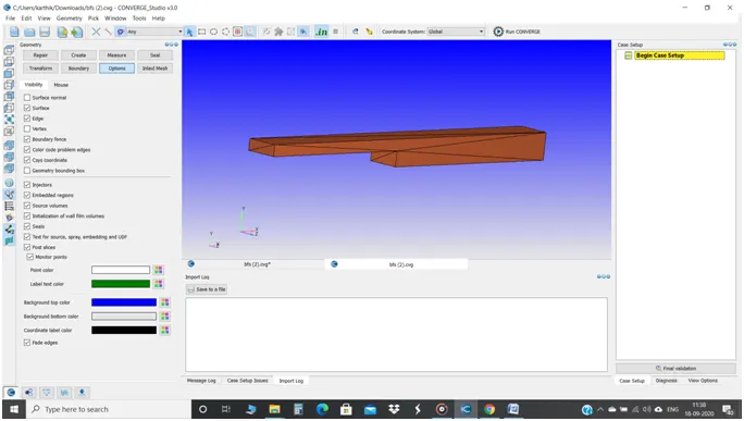
• It is better to check the case initially that how it’s been scaled. To ensure that, Click Options and under the tab of Visibility, click Geometry Bounding box to create Boundary line across the geometry and to check the geometry dimension.
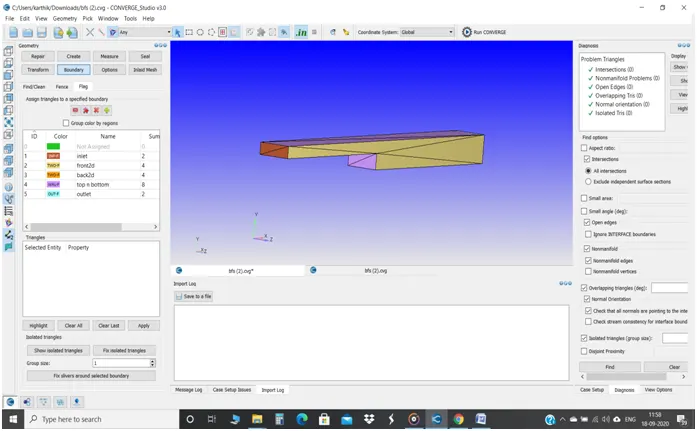
• After that, to ensure that whether the geometry is clean or not, click Diagnosis tab and click the normal checking option in order to ensure that all the normal orientation are pointed towards the direction of flow of fluid and click Find.
• To create a boundary surfaces, make sure cursor picks the Triangle
• Select Boundary, in the Flag tab, click + to add the boundaries.
• Add the boundaries by clicking create multiple boundaries to create all the boundaries at a once and name them like Inlet, Outlet, Top and bottom walls, front 2D and back 2D by selecting the respective triangles and click Apply.

• In order to begin the case setup, click case setup and click begin case setup and click Time Based, since it is not a crank angle based like lC engine or Pumps but a steady state channel flow setup.
• By clicking Materials, select Air to be predefined mixtures.
• In Simulation Parameters, under Run Parameters in Solver tab fix the solver to be Steady state solver, the simulation mode to be Full Hydrodynamic, since no need to create mesh by No Hydrodynamic and it is also not a complex setup and it didn’t take much time for running simulations.
• In Miscellaneous tab, check the steady state monitor and uncheck the Use Shared memory because of we are running a steady state simulation flow.
• In Boundary conditions, name the respective Boundary type like Inlet as Inflow, Outlet as Outflow, Top and bottom walls to be wall of No-slip, Front and back as Two-D.
• In inlet, in Pressure boundary conditions, select the Specified value to let the inlet pressure be 110000 Pa and select the predefined mixture as Air which contains N2 as 0.77 and O2 as 0.23 and select the temperature to be specified value of 300 K and Outflow as 100000 Pa.
• Make sure the inlet pressure is higher than outlet pressure.
• Since we checked the Steady state monitor, in the steady state monitor, click Add config. And click Add to add the variables that needs to be monitored in the simulation.
• In Simulation time parameters, under General tab, the End time is 16000 cyc. The initial and minimum time-step is 1e-9 and end time is 1 sec and click ok and click ok on Solver parameters with default values.
• In Regions and Initialization, click Add as Region 0 and set pressure as 101325 Pa (atmospheric pressure) since the flow shouldn’t get reversed and click Air as its Species.
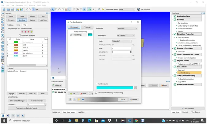
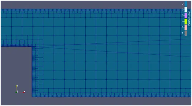
• Then in Grid control, a unique kind of meshing system is introduced which is called Fixed Embedding. The mesh size that want to be created is typed in metres.
• First case as 2e-3m, second case as 1.5e-3m, third case as 1e-3m.
• As we choose Fixed embedding, in that option, click Add and entity type as Boundary, the Boundary ID as Top and Bottom walls (where the mesh of fixed embedding will be created) and the scale of mesh as 3 and the Embed layer is 1 and the Mode as Permanent and click ok.
• Fixed Embedding is nothing but the refining system of mesh in particular boundary with respect to the scale.

• Then in Post variable Selection, click on Species/Passive, check the Mass fraction and add the N2 and O2.
• For Output Files, Time interval for writing 3D output files is 100 cycles which is the time interval between the one and another output file that get dumped in output files successively and the maximum no. of restart files that saved is 3 which is a Factor Of Safety and click ok.
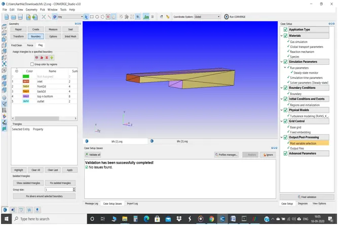
• Now, when we click on Validate all options for validating , we could see that everything has been validated and checked as foll. Picture:

Simulation by CYGWIN:

• Once the case setup is ready, the input files has been exported to the particular location and the copy and paste the mpiexec.exe file in that location.
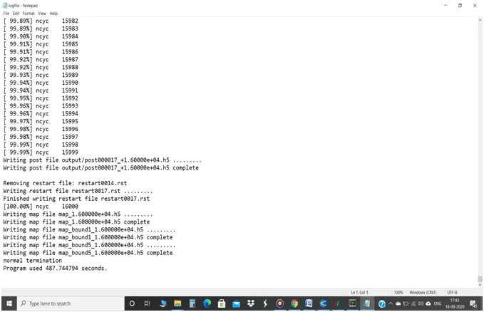
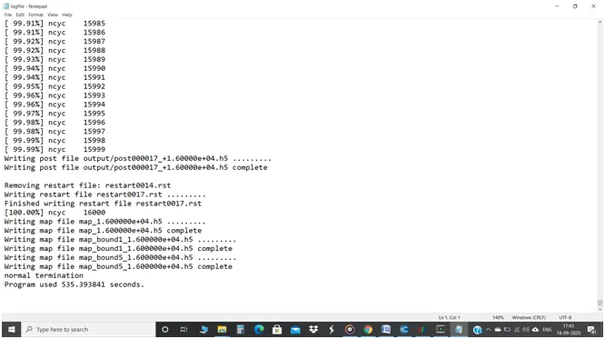
• Then, the input files have been simulated in CYGWIN and we can see the total time taken for the simulation.

For the mesh size 2e-03m:

For Mesh size 1.5e-03:

For Mesh size 1e-03:

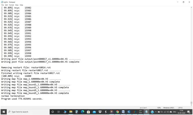
• It is denoted that time taken for the simulation of entire backward flow step setup for the base mesh size 2e-03 is about 487 seconds and for base mesh size 1.5e-03 is about 535 seconds and for base mesh size 1e-03 is about 774 seconds.
• Eventually, the amount of mesh size gets smaller or the number of cells gets higher, the amount of time taken for the simulation gets higher.

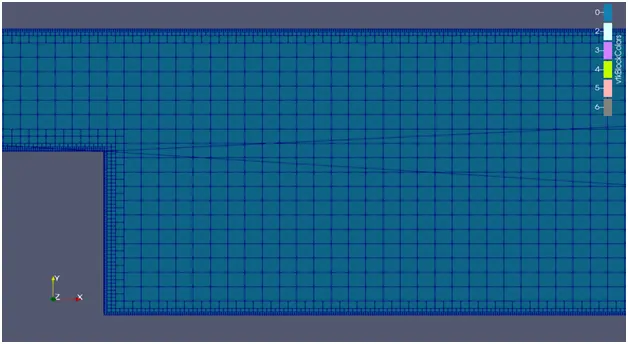
Surface mesh:

Mesh size 2e-03m:

Mesh size of 1.5e-03m:

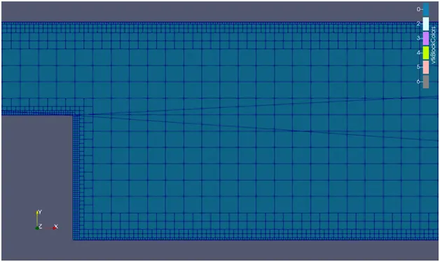
Mesh size of 1e-03m:

Analyzing the plots in Converge CFD:

For Mesh size 2e-03:

Velocity plot:

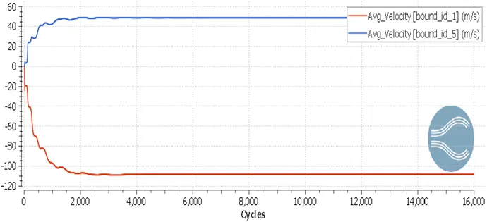
• Here, at inlet, from this graph, the velocity is reached up to 110m/s approx. and at outlet the velocity is reached up to 50m/s approx.
• The velocity at the inlet is higher than the velocity at the outlet. This is due to the (sudden) expansion in the area of the flow of the fluid, since, the area is inversely proportional to the velocity (A=k/V)
• Then, the cycle is seemed to exactly got converged at 4000 cycles with some slight crests and troughs between 2000 and 4000 cycles.

Pressure plot:

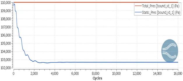
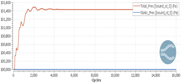
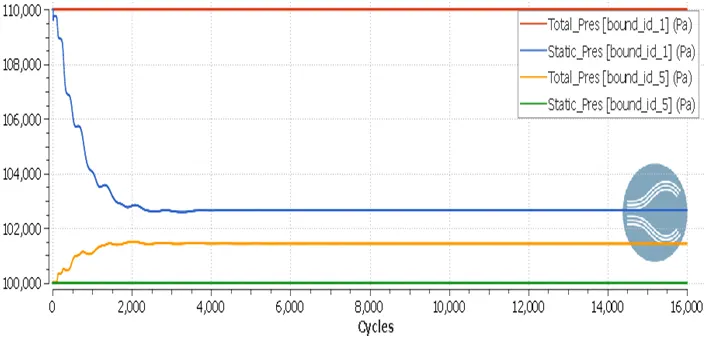
• Here in the pressure plot, the value of Total pressure and static pressure is same at initially because the pressure of fluid that is not moving (Static pressure) is equal to total pressure (Static pressure + dynamic pressure), which also means dynamic pressure is zero.
• As the cycles going on, the static pressure is getting decreased (up to 102660 Pa) with the fluctuations (due to expansion in area) due to increase in dynamic
• At the outlet, the static pressure will be 100000 Pa and the total pressure value is increasing to 101430 Pa with respect to cycles due to increase in dynamic pressure.

Mass flow rate:

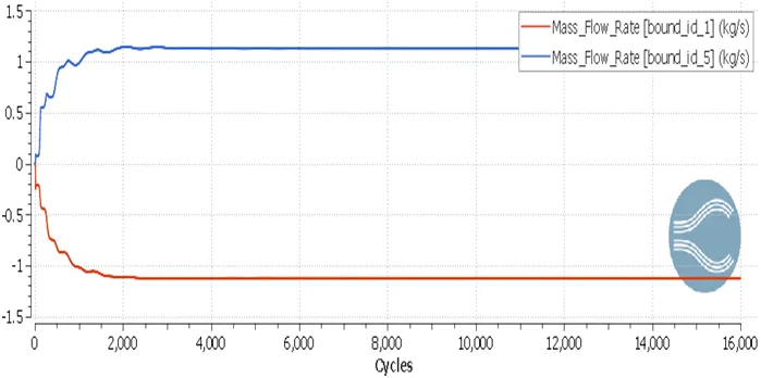
• Mass flow rate is defined as the mass of the substance which passes per unit time.
• From the graph, at both the inlet and outlet, the mass flow rate increases up to 1.12 kg/s with the fluctuations that caused by expansion in area.
• The Mass flow rate value gets the same value around 3000 cycles.

Total Cell count:

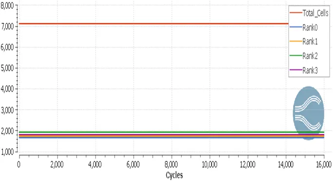
• From the graph, the total cell counts has been shown and used is 7000 cells. It also to be noted that we have been used 4 processors from rank 0, rank 1, rank 2, rank 3.

For mesh size 1.5e-03:

Velocity plot:

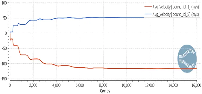
• From this graph, at inlet (bound_1), the velocity has reached up to 115m/s and at the outlet, the velocity is 50m/s approx.
• Due to the increase in area only, the value of the outlet velocity is low. But the no. of cycles to get converged is higher than the mesh size 2e-03 m.

Pressure plot:

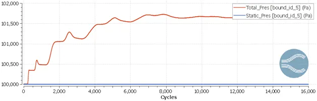
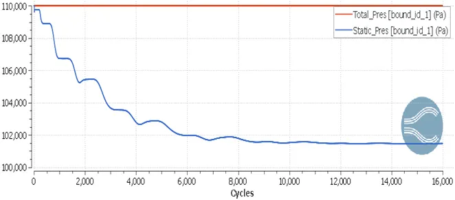
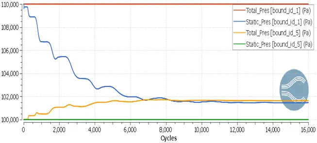
• From the graph, the decrease in static pressure and the increase in total pressure reacts in high rate than the mesh size 2e-03.
• The static pressure at , decreases to 101480 Pa and the total pressure increases to 101640 Pa.
• It seems that there is a lot of fluctuations in pressure at the area of expansion.

Mass flow rate:

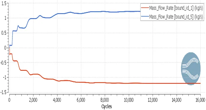
• Here at both the inlet and outlet, the mass flow rate gets the same value of about 1.20kg/s with the slight + or - 2 kg/s deviation at around 8000 cycles.

Total cell counts:

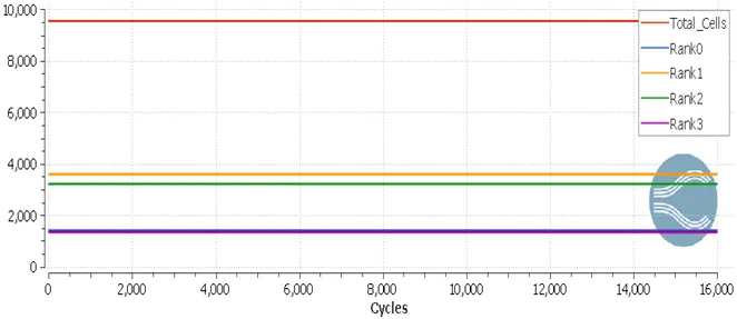
• The total cell counts of mesh size 1.5e-03 is around 9600 cells.

For mesh size 1e-03:

Velocity plot:

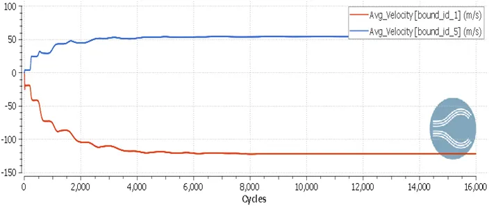
• In this case, at inlet, the velocity is 122m/s and at outlet the velocity is 53m/s.
• From the graph, it shows that the flow has been converged around after 10000 cycles.

Pressure plot:

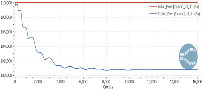
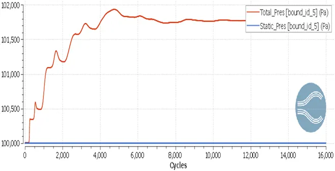
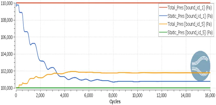
• When comparing to remaining mesh sizes, it gives more exact and higher value of pressure.
• At outlet, the value of total pressure reaches up to 101773 Pa and the static pressure, at inlet, decreases up to 100754 Pa.

Mass flow rate:

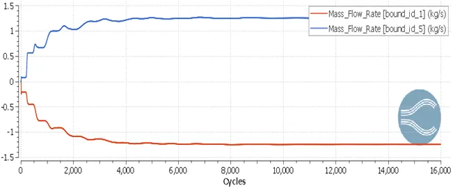
• From the graph, Mass flow rate of mesh size 1e-03 gets the maximum value of about 1.25kg/s.

Total cell counts:

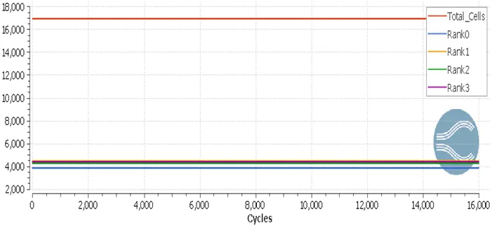
• The total cell count that can be achieved with mesh size of 1e-03 is 16900 cells.

Analyzing the fluid flow using PARAVIEW:

• Backward facing step is a benchmark geometry used for several specific purposes where the flow experiences several flow characteristics.

Initially, the static pressure is high and zero velocity condition as following picture:

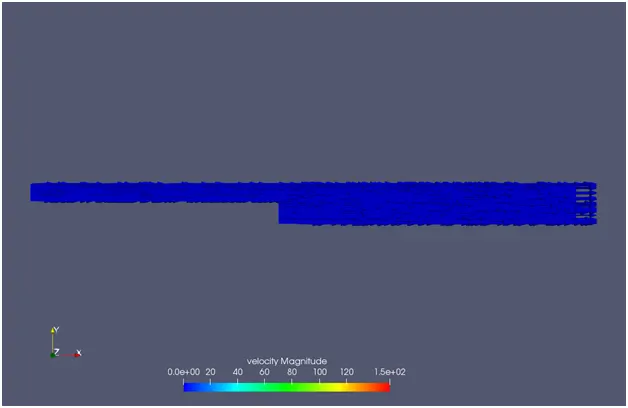
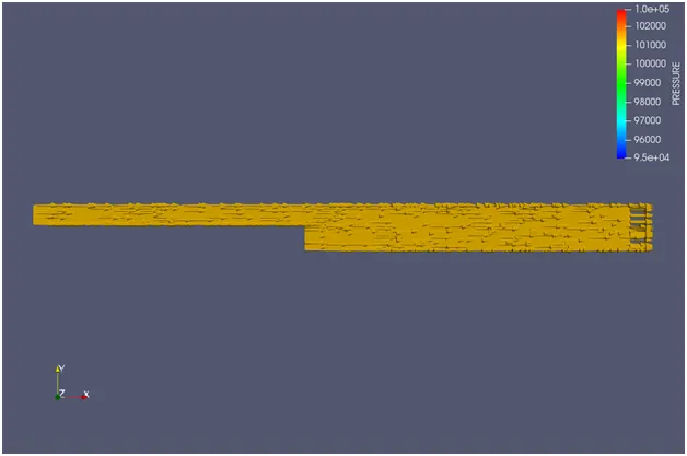
• The general flow of Backward facing step starts with the upstream boundary layer with high velocity.
• Then, the flow gets separating at the step edge and can be divided into three parts named as Shear layer region, recirculation zone and reattachment zone.
• As the flow separates, initially, the shear layer gets developed (by streaming downwards) due to the area expansion. The region where the flow of shear layer develops is known as Shear Layer region(the shear layer that will be created here is Free shear layer).
• The Primary vortices, which creates from the turbulent flow of shear layer region by getting away from that region and the secondary vortices, which creates due to the corner step at the adjacent of it collectively combines a zone called Recirculation zone.
• The flow of shear layer then streams downwards and hits at a point called Reattachment point and the length between the step and reattachment point is called reattachment length and it expands for some small distance called reattachment zone.
• After it reaches the reattachment zone, it forms a new shear sub-boundary layer and rapidly gets distorted which deflected the flow to travel upstream and results in fluctuations of velocity within the shear layer.

Velocity contour:

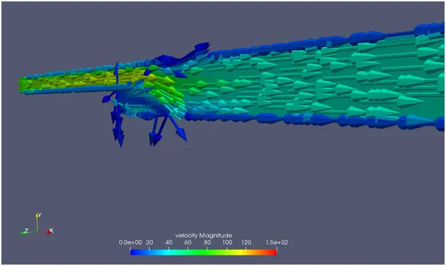
At Initial cycles:

Mesh size 2e-03m:

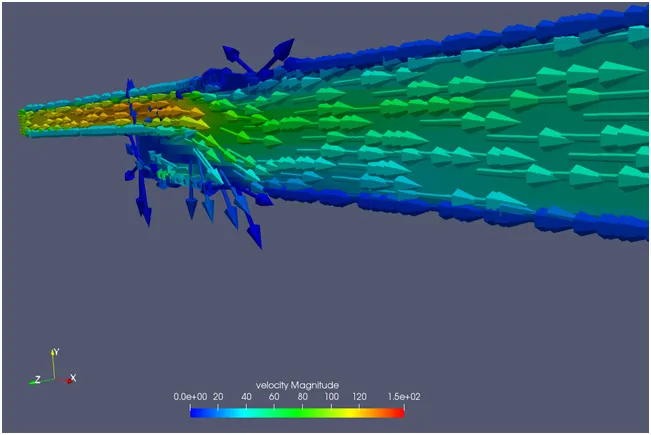
For Mesh size 1.5e-03:

For mesh size 1e-03m:

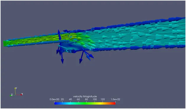
• The value of velocity, from the inlet to reattachment zone, of the mesh size 2e-03m>1.5e-03m>1e-03m.
• At the recirculation zone, the velocity is smaller in the mesh size of 1e-03m>1.5e-03m>2e-03m.
• It is also to be noted that the reattachment length is smaller in 1e-03m>1.5e-03m>2e-03m.
• It has to be noted that the reattachment point has touched the bottom wall only in mesh size of 1e-03m but in the remaining mesh sizes it doesn’t, just got deflected within the geometry case.

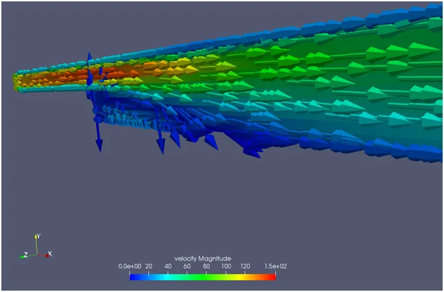
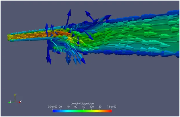
After some cycles :

For mesh size: 2e-03m:

For mesh size 1.5e-03m:

For mesh size 1e-03m: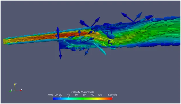

• After some cycles, the velocity at the separation stage has increased.
• And, the deflected upstream from the reattachment point can be noted.
• The flow can be clearly viewed and analyzed by seeing the mesh of 1e-03m.

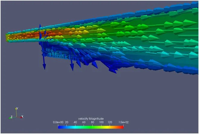
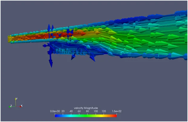
At the level of convergence:

For mesh size 2e-03m:

For mesh size 1.5e-03m:

For mesh size 1e-03m:

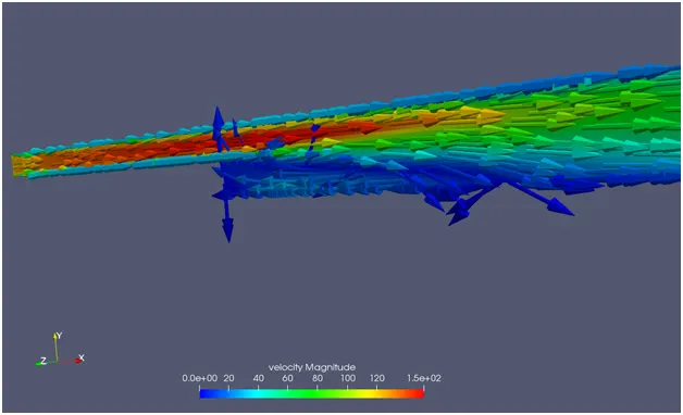
• At the level of convergence, the velocity at the separation stage gets even more higher and after that gradually, becomes less and leaves the outlet
• The value of velocity is much clear only at the the mesh size 1e-03m.

Pressure Contour:

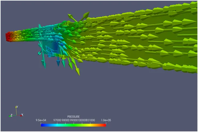
At initial cycles:

For mesh size 2e-03:

For mesh size 1.5e-03m:

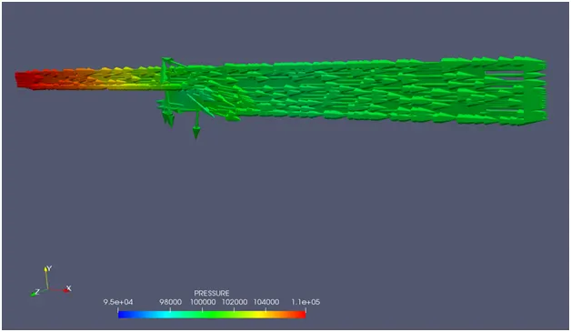
For mesh size 2e-03m:

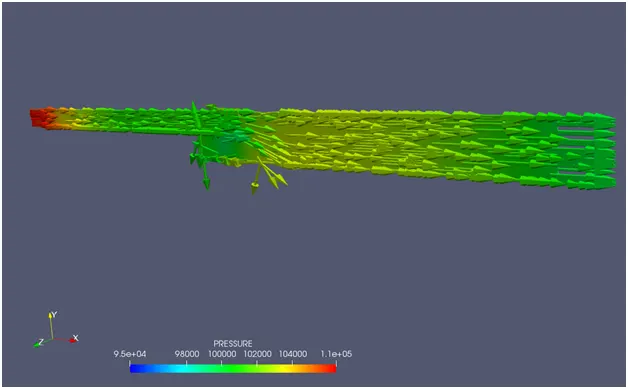
• At inlet, in all the three cases, static pressure is high.
• It just getting decreased at the area of separation due to the area expansion.

After some cycles:

For mesh size 2e-03m:

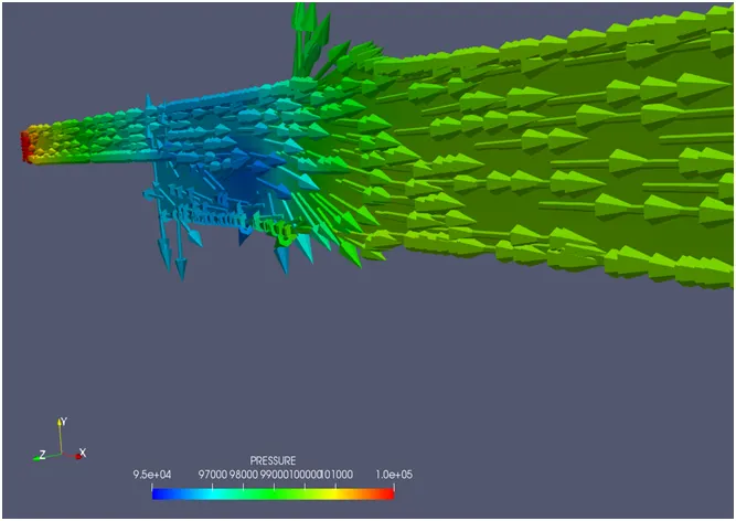
For mesh size 1.5e-03:

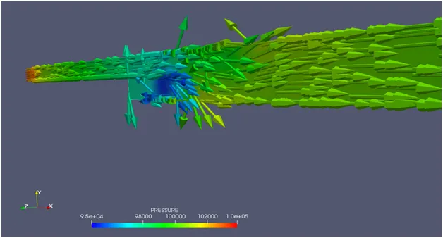
For mesh size 1e-03m:

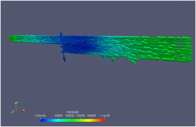
• As the cycles gets increasing, the static pressure is decreasing due to the increase in dynamic pressure.
• At the area of Recirculation zone, the pressure is very low since there is only primary vortices and secondary vortices and it didn’t go beyond 98000 Pa there.
• The pressure, at the outlet, is almost in the green region, so the pressure is almost less than the inlet due to the expansion in area.

At the level of convergence:

For mesh size 2e-03m:

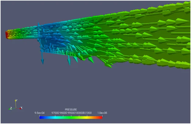
For mesh size 1.5e-03m:

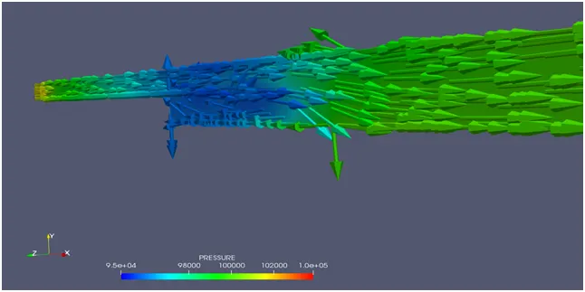
For mesh size 1e-03m:

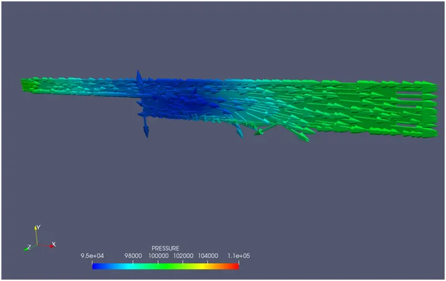
• At the final cycles or level of convergence, since the mesh size of 1e-03 gives the finer value, it looks that static pressure gets decreased at the inlet and in the green region.
• At the area of separation, the static pressure is completely decreased and just reaches the blue region.
• At the area of the outlet, the pressure just remains in the green region which also means maintains at the same level approximately.

Conclusion:

1. As the mesh size or the total number of cell counts gets smaller, the physical results of simulation through PARAVIEW and the numerical results through plots in Converge CFD gets more exactly or the results are trying to get a exact value of the flow.
2. The flow simulation of Backward facing step leads us to understand about the creation of vortices and turbulent flows and the purpose of simulating it and its applications and several concepts of CFD like recirculation zone, reattachment zone.
3. Adding the mass fraction of N2 and O2 tends to get clear view of the simulation of backward facing step in PARAVIEW.
4. The purpose and idea of making Fixed embedding which is a nice feature to have when you know exactly where the added mesh will be needed.

Links for animations:

For mesh size 2e-03m:

velocity animation: https://www.youtube.com/watch?v=4nheozRAMuo

pressure animation: https://www.youtube.com/watch?v=G-x80Soonl0

For mesh size 1.5e-03m:

velocity animation: https://www.youtube.com/watch?v=eHHfAnvL32Q

Pressure animation: https://www.youtube.com/watch?v=rYvuyc92-Xg

For mesh size 1e-03m:

Velocity animation: https://www.youtube.com/watch?v=rttvpoODIns

Pressure animation: https://www.youtube.com/watch?v=CQuG-dy0liE