Week 7 - CHT Analysis on a Graphics card
Aim: To run Conjugate Heat Transfer Analysis of a Graphics Card in Ansys FLUENT.
Introduction and Practical Significance:
Graphics Card is among the parts in a computer, which are subjected to higher heat loads. This is due to the heat dissipiated by the processors continiously. This heat is required to be removed fromt these units otherwise these critical parts can fail easily from accumulated thermal stresses and even by melting of sub components. The bigger the processor the greater is its power consumption and as a matter of fact 99.99% of power consumed by the processor is dissipiated as heat [1]. This is an an engineering design challenge, since we can not change the fundamental thermodynamics of processor, we must manage the heat load. Thus, fans and even coolants are incorporated in computers to tackle this issue. We won't be considering the flow through fan but we will try to heighlight the thermal management of a Graphics Card through flow of air around it and how rate of heat transfer is dependent on the flow velocity and also the properties of materials used in a graphics card.
Theorey:
Because of the nature of Heat Transfer process Conjugate Heat Transfer Analysis is required. The overall Heat transfer is obtained by convection between the parts of the graphics card and fluid flowing around it, as governed by Newton's Law of Cooling, then in between the solid parts of graphics card through conduction, which is Governed by Fourier's Law of Heat Conduction.
Fourier's Law of Heat Conduction:
According to this law the rate of Heat flux is directly proportional to gradient of temperature in Space
d/dt (q/A) ∝ ∇.T
= -k ∇.T
where, k is constant of proportionality called thermal conductivity of the material which is a property of solid. [w/mK] q is the amount of heat transfered [j]
Newtons Law of Cooling:
The rate of heat flux between a flowing fluid and stationary solid is given by,
d/dt (q/A) ∝ (T(fluid) - T(solid))
= -h*A*(T(fluid) - T(solid))
where, h is constant of proportionality called convection heat transfet coefficient. [w/mK]
h = f(thermophysical properties of the fluid, velocity of the fluid)
=> if anywhere in the computational domain velocity increases, the heat transfer coefficient must also increase
Solving and Modelling Approach:
We have a simplified model of a graphics card so that we can focus on the fundamental physics incorporated behind its design. The real and practical models are hard for topological cleanup for CFD and thus working on a realistic model is a time consuming task. So in our model, air flows around it and the heat which is generated by the processor is getting dissipiated, its our task to determine how this heat is getting distributed and how is heat transfer coefficient getting affected by the flow velocity.
We are going to take the following steps to complete this problem:-
1. Working on Base-line Mesh:
Here, we will use the default settings and run the simulation to see what needs to be improved.
2. Refining the Mesh until Mesh Independence = Mesh Independence Test:
Now, we will keep refining the mesh until our results get consistent and most importantly, independent of mesh Refinement.
4. Test of Convergence
Once Quality Mesh and proper solver settings are established we will test the accuracy of solution through test of convergence.
5. Running all Cases on Finalised Mesh and Sover Settings:
Our task involves running the simulation on varying velocities, so we will use the best mesh obtained to run all these cases. This way we will try to underpin the dependence of heat transfer coefficient on Velocity of flow.
Every setup is going to involve the below mentioned steps:
1. Preprocessor and Solver Settings:
2. Running Simulation
3. Post Processing the Results
Baseline Simulation
1. Pre Processing
1.1 Geometry Setup in Space Claim
Here we will put the geometry in space claim and in order to generate conformal mesh we must use Share Topology feature in Space Claim
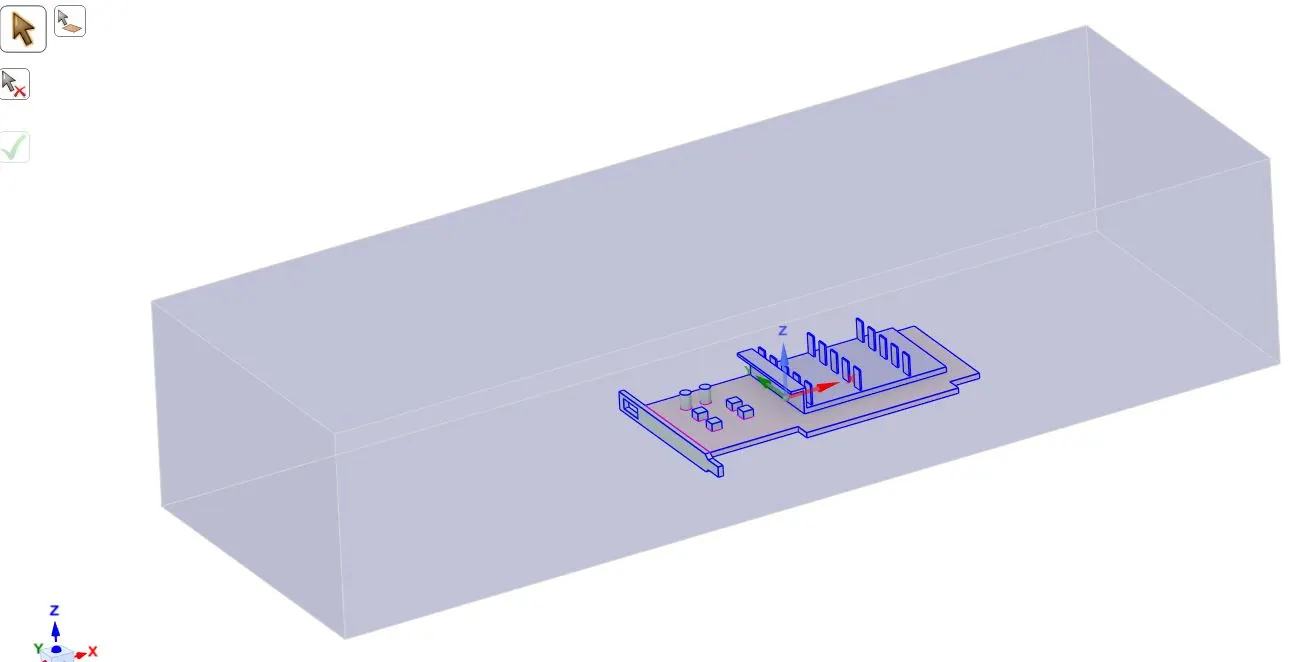
Fig 1: Geometry setup in SpaceClaim
1.2 Mesh Generation In Ansys Mesher
We will generate the baseline mesh based on the default settings which is CFD based tetrahedral Mesh.
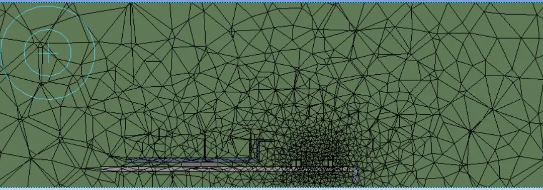
Fig 2: Baseline Mesh
Element Quality average for the whole mesh == 81%
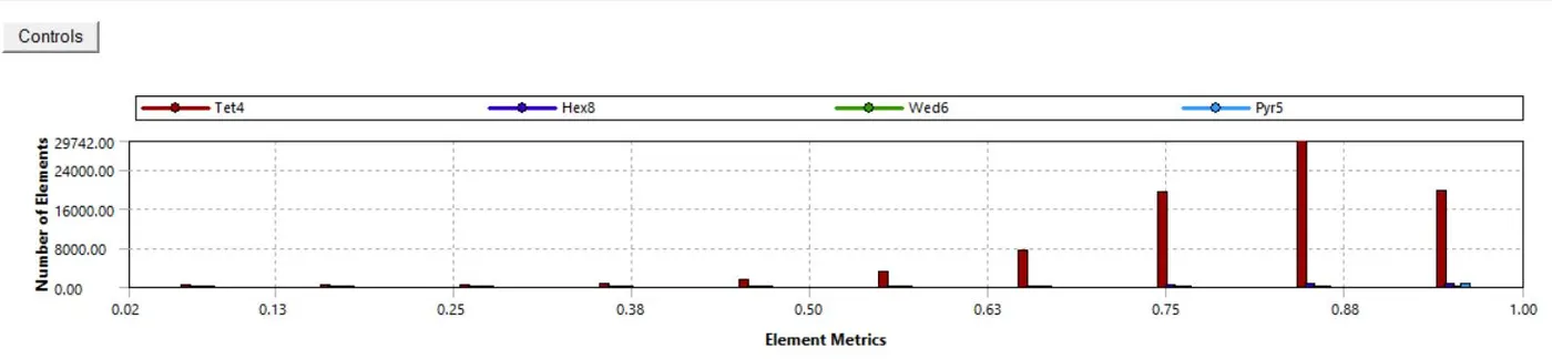
Fig 3: Element Quality or Mesh Metric for Baseline Mesh
Statistics:
Total Number of Nodes = 15658
Total Number of Elements = 83464
Average Element Quality = 81.09%
2. Solver Settings
Now we will setup the basic setup before proceeding to solver.
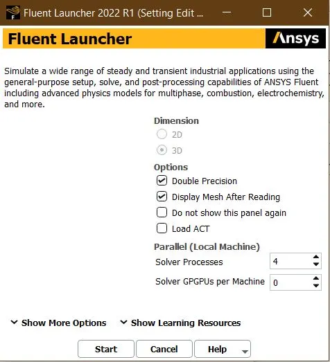
Fig 4: Fluent Settup
3. Running Simulation
General Setup
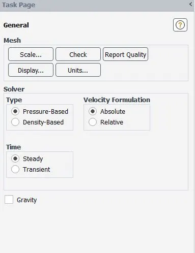
Fig 5: General Fluent Settings
We need to first setup the Viscous Model.
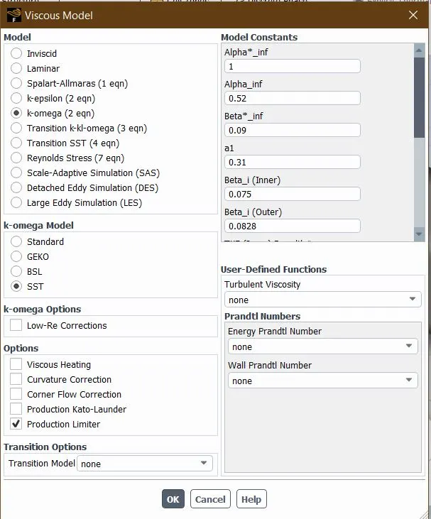
Fig 6: Viscous Model Setup-Default
Now we have to set up the Material Properties and Cell Zone Conditions for Each Part of Graphics Card
Air for Enclosure
Material Properties
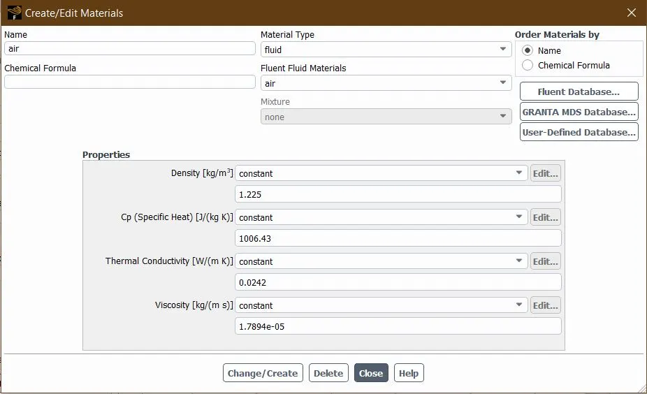
Fig 7: Material Properties-Air
Cell Zone Conditions
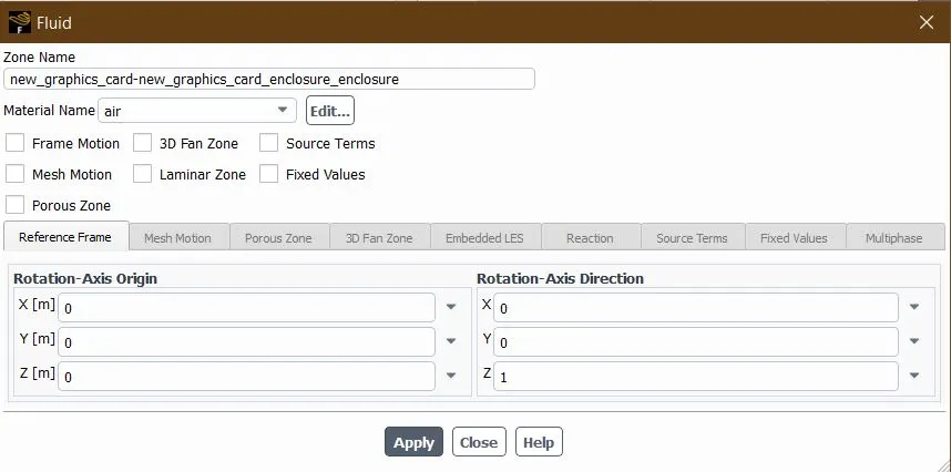
Fig 8: Cell Zone Conditions-Air
Aluminum for Fins
Material Properties
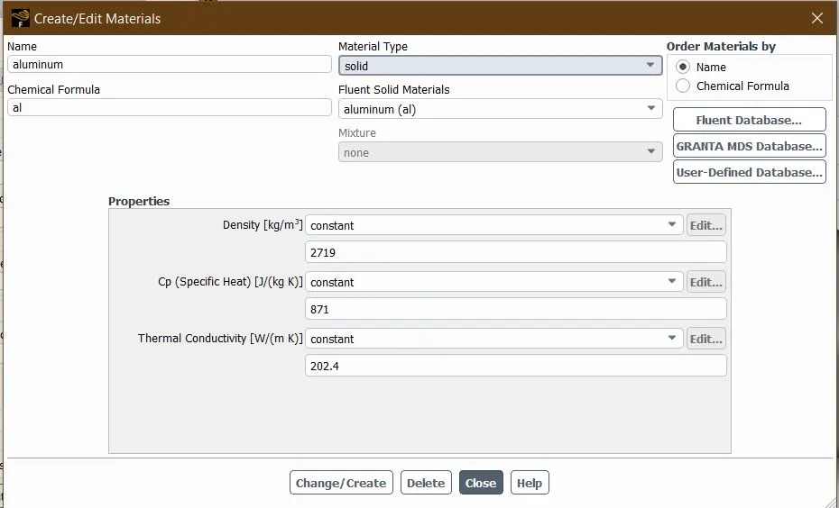
Fig 9: Material Properties-Aluminium
Cell Zone Conditions
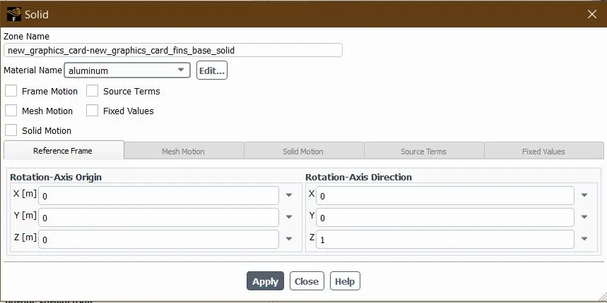
fig 10: Cell Zone Conditions-Aluminum
Fr4 for Base
Material Properties
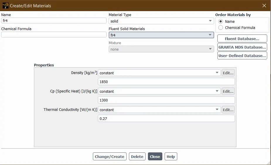
Fig 11: Material Properties-FR4
Cell Zone Conditions
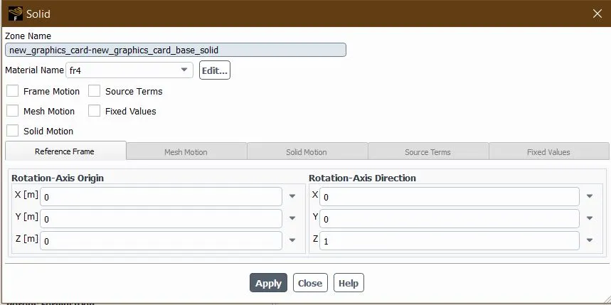
Fig 12: Cell Zone Conditions-FR4
Silicon for Processor
Material Properties
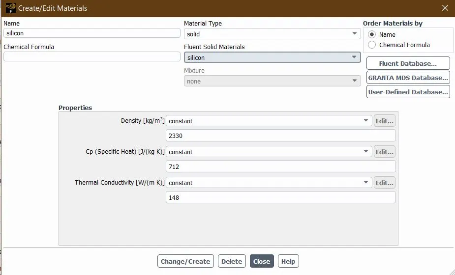
Fig 13: Material Properties-Silicon
Cell Zone Conditions
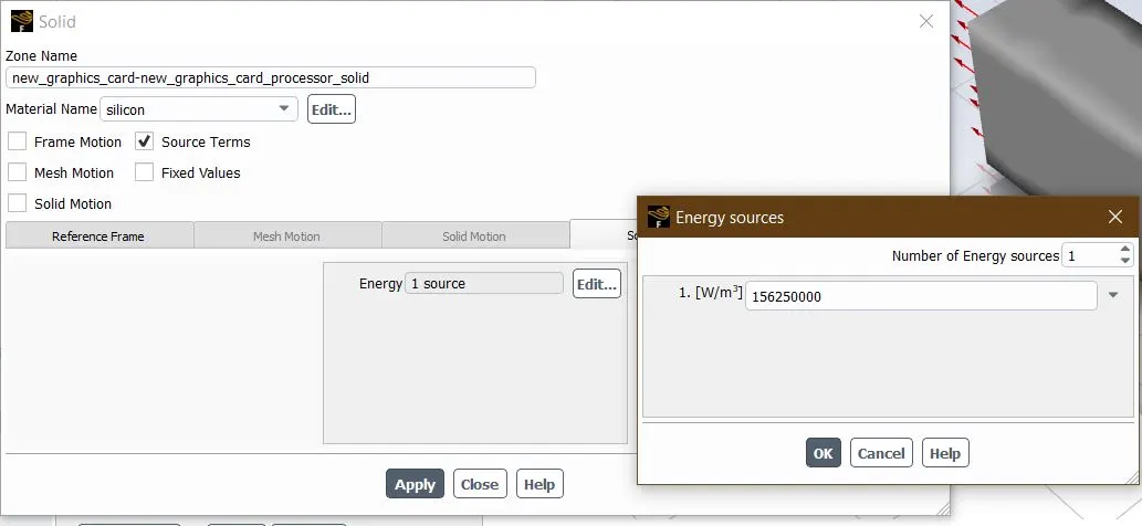
Fig 14: Cell Zone Conditions- Silicon
Heat Generation Calculations
For Processor we will provide with a source of heat.
Power = 10 W
Volume = 8*8*1 = 64 mm^3
Heat Generation / unit Volume = 1.5625 *10^8 W/m^3
Solver Settings:
We are going to use default settings
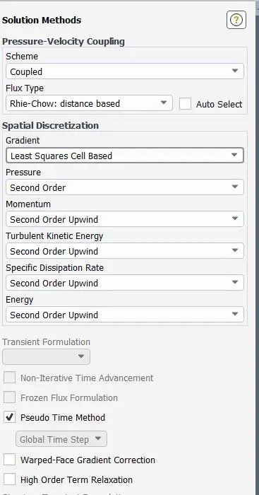
Fig 15: Default Solver Settings
We will also use the default Under Relaxation Factors
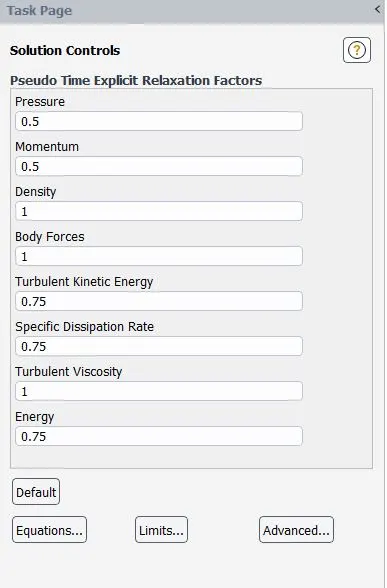
Fig 16: Relaxation Factors
Results Obtained
1. Residuals
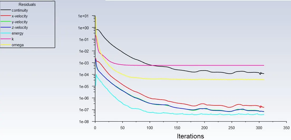
Fig 17: Residuals for Baseline Mesh
As we can see the residuals are not depicting a properly converged solution
2. Temperature Contours
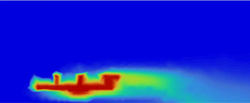
Fig 18: Temperature Contours for Baseline Mesh
As we can see the contours of temperature are too blurred and thus refining of mesh is essential before proceeding to a Results discussion. As observed, the region around graphics card is very crucial for heat transfer and thus it must be properly and selectively refined. For this purpose we are going to incorporate Multi Zone Approach.
Mesh Independence Test
We will refine the mesh step by step and when the variables obtained show consistency in values, we will declare our mesh as independent of refinement.
Refined Mesh 1
Outer Enclosure Element size = 5mm
Inner Enclosure Element Size = 1mm
Graphics Card Element Size = 0.5mm
Mesh
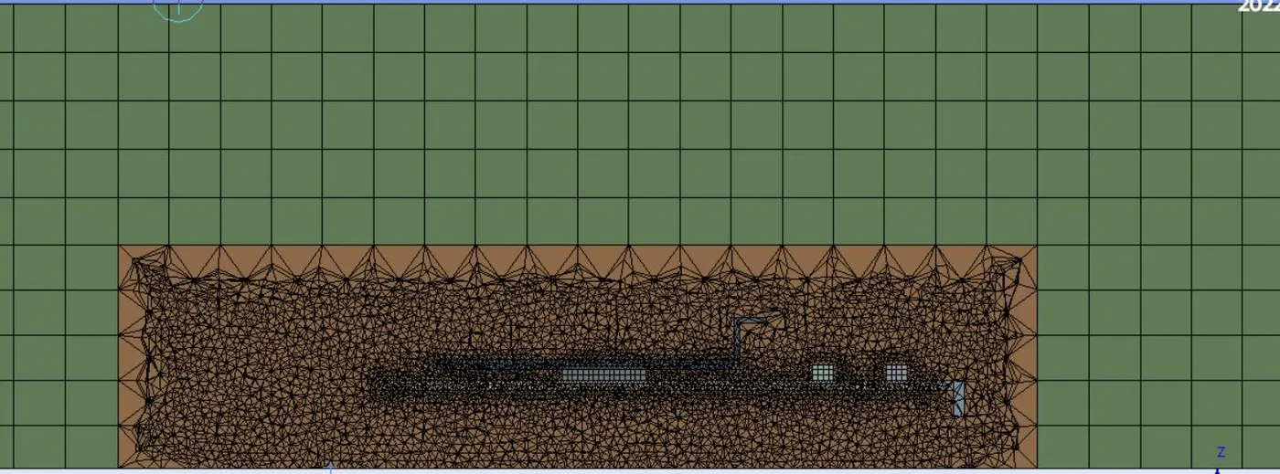
Fig 19: Refined Mesh 1
Statistics:
Total Number of Nodes = 146832
Total Number of Elements = 835429
Average Element Quality = 80.74%
Element Quality
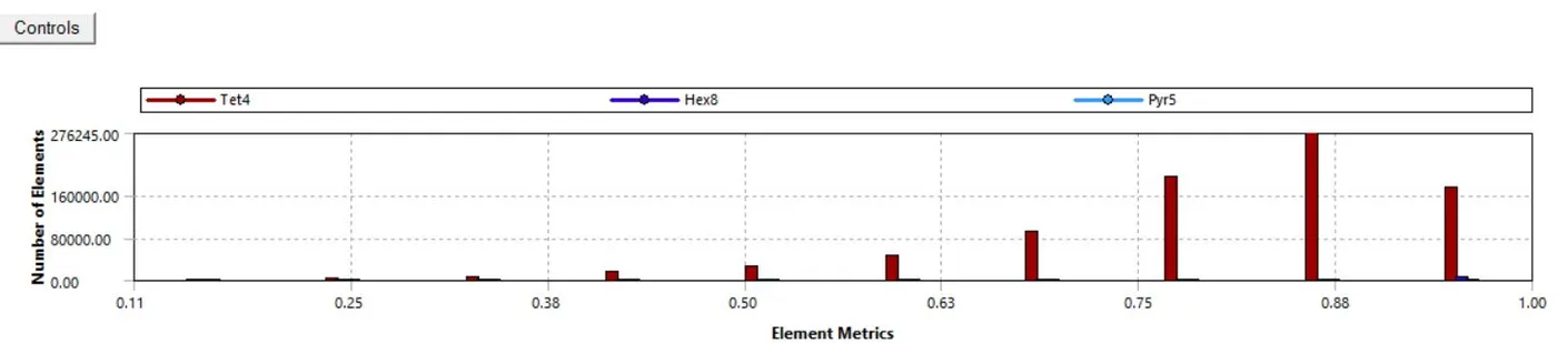
Fig 20: Element Quality for Refined Mesh 1
Residuals
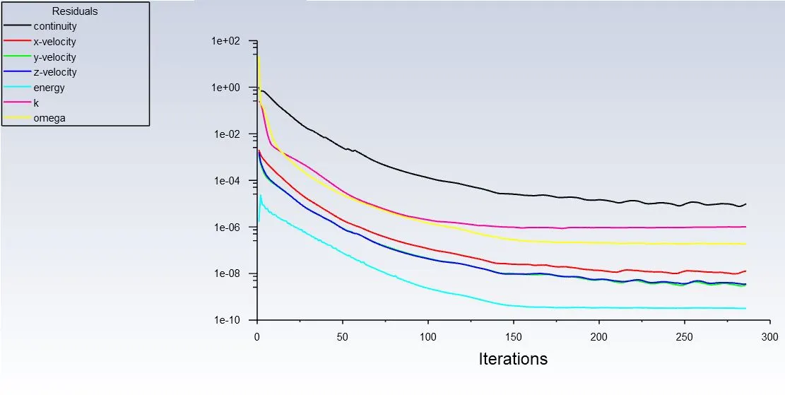
Fig 21: Residuals for Refined Mesh 2 == 1e-4
Temperature Contours
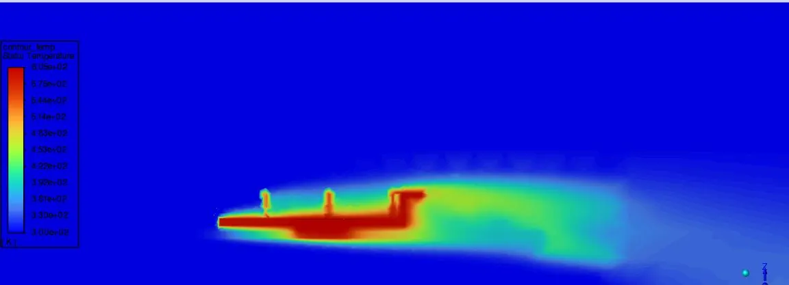
Fig 22: Temperature Contours for Refined Mesh 1
As we refined the mesh we saw that residuals droped considerably lower and also contours of Temperature improved significantly.
Refined Mesh 2
Outer Enclosure Element size = 3mm
Inner Enclosure Element Size = 1mm
Graphics Card Element Size = 0.25mm
Mesh
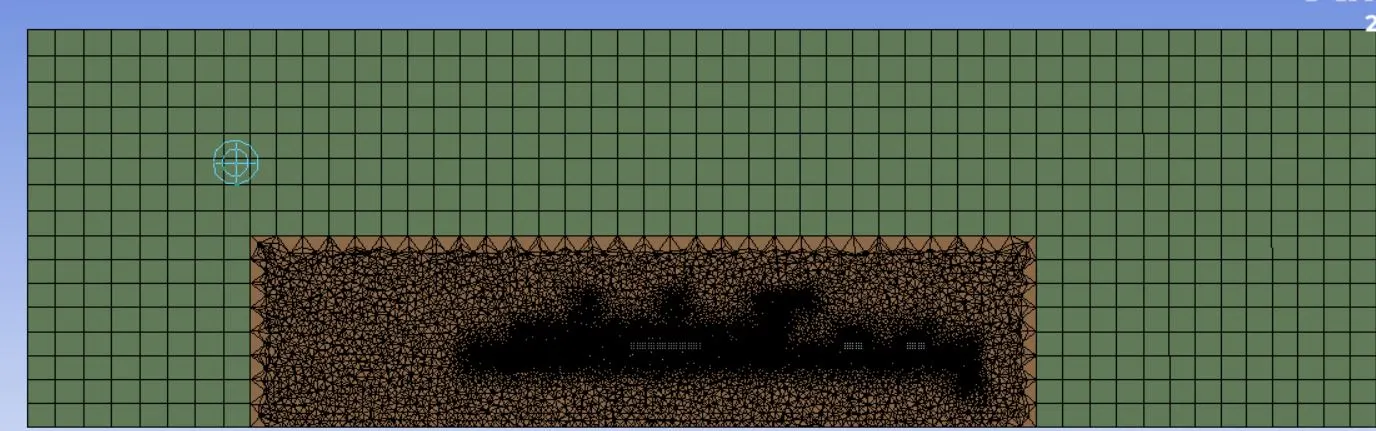
Fig 23: Mesh for Refined Mesh 2
Statistics:
Total Number of Nodes = 606123
Total Number of Elements = 3475044
Average Element Quality = 83.37%
Element Quality
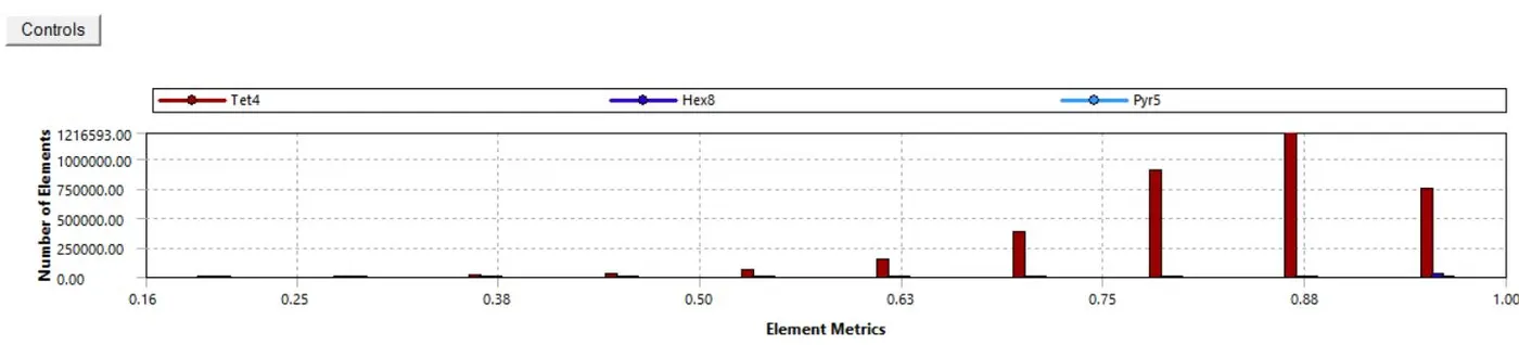
Fig 24: Element Quality for Refined Mesh 2
Residuals
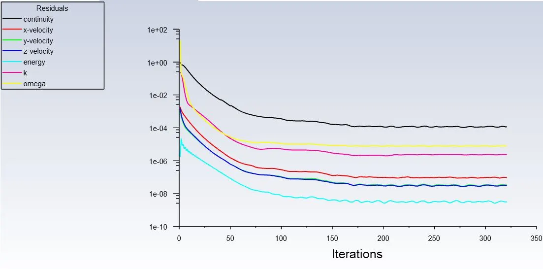
Fig 25: Residuals for Refined Mesh 2 1e-3
Temperature Contours
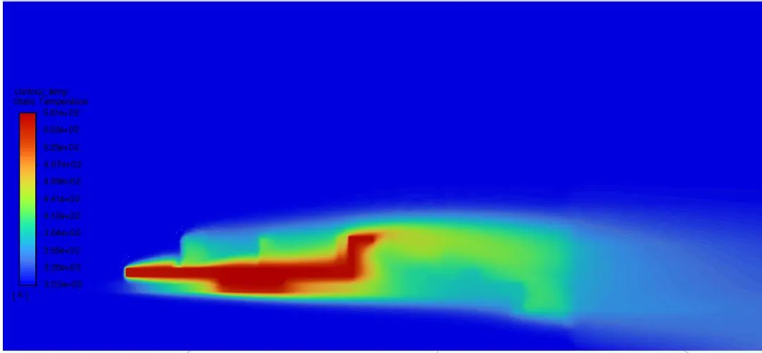
Fig 26: Temperature Contours for Refined Mesh 2
Refined Mesh 3
Outer Enclosure Element size = 3mm
Inner Enclosure Element Size = 0.75mm
Graphics Card Element Size = 0.2mm
Mesh
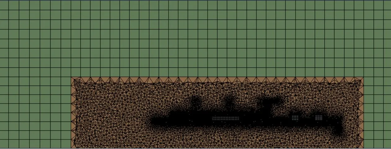
Fig 27: Mesh for Refined Mesh 3
Statistics:
Total Number of Nodes = 941376
Total Number of Elements = 5455053
Average Element Quality = 83.48%
Element Quality
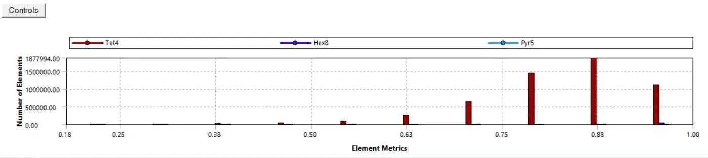
Fig 28: Element Quality for Refined Mesh 3
Residuals
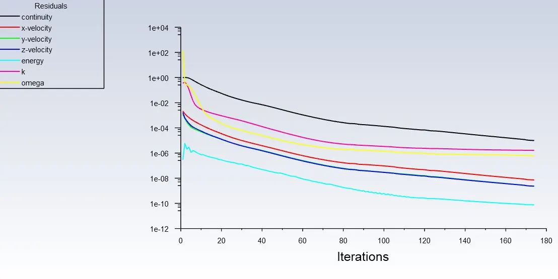
Fig 29: Residuals for Refined Mesh 3 1e-6
Temperature Contours
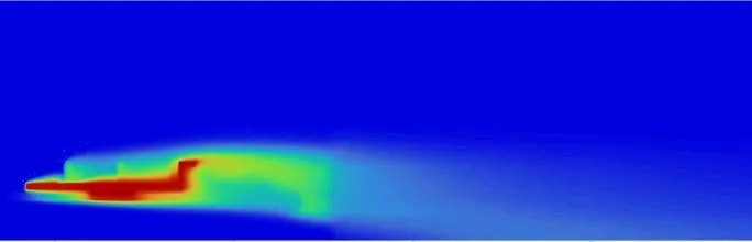
Fig 30: Temperature Contours for refined mesh 3
Mesh Independence Test Summary
| Baseline | Refined 1 | Refined 2 | Refined 3 | |
| Surface Heat Transfer Coefficient at Processor [W/m^2K] | 5.397 | 6.309 | 6.589 | 6.643 |
| Surface Heat Transfer Coefficient at Fins[W/m^2K} | 15.96 | 18.283 | 19.571 | 19.618 |
| Temperature at Processor[K] | 514.343 | 593.664 | 579.304 | 578.74 |
| Temperature at Fins[K] | 508.435 | 590.95 | 572.779 | 572.073 |
Table 1: Summary of Mesh Independence Test
Mesh Independence Test Conclusion
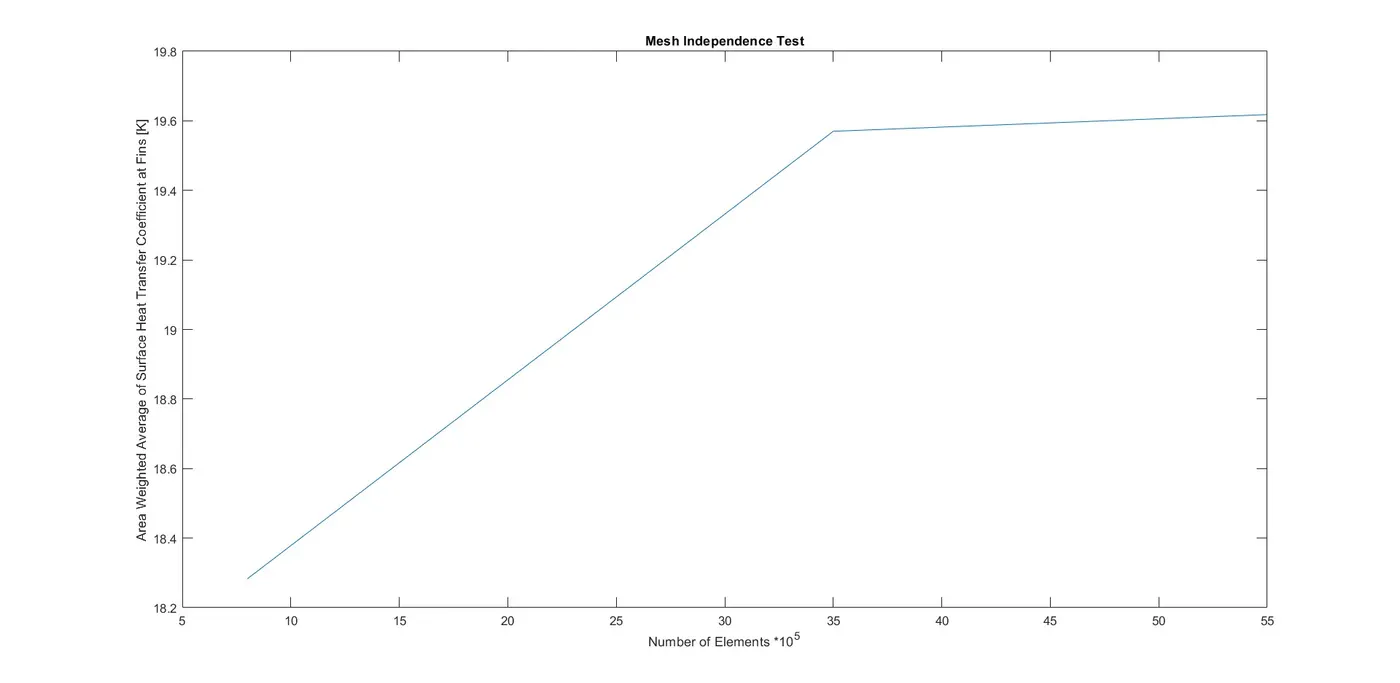
Fig 31: shtc vs Number of Elements
As we can see Surface Heat Transfer Coefficient at Fins is not varying significantly and thus Mesh Independence Test is achieved.
Convergence Test
Convergence referes to the stability of a numerically solved partial differential Equation, from a mathematical point of view. But the defination is not limited under the spectrum of mathematics only. For instance a solution which reflects the physical principles is also considered as a converged solution. Hence, speaking broadly there are mainly two ways to demonstrate convergence of a solution:
1. Mathematical Convergence:
Generally, if residuals are below 1e-3, then such solution is considered converged mathematicall. It reflects the invarience of values across the elements and is a strong function of Mesh Quality.
Fig 32: Residuals convergings below 1e-6
As our residuals are well below 1e-3, we can proclaim that our solution is converged mathematically.
2. Physical Convergence:
A solution is converged Physically when it reflects the expected physical behaviour. When it is about problems on Heat Transefer Analysis, we can demonstrate convergence by Energy Balance, if the value is very close to zero, then solution is considered converged physically.
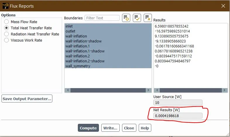
Fig 33: Energy Balance
As we can see the net rate change of heat == 0. Thus validating physical convergence.
Case 1: V = 1 m/s
We will now use the steps and solver settings involved in Refined Mesh 3 and explain the results.
1. Residuals
Fig 32: Residuals for V= 1 m/s
2. Area Weighted Average of Temperature at Processor = 578.74 K
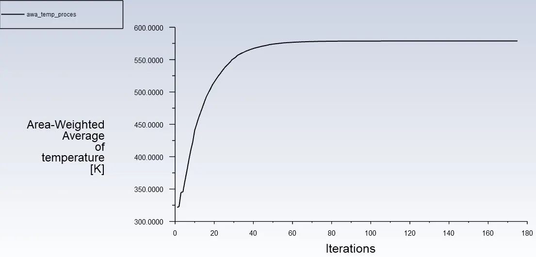
Fig 33: Temperature at Processor
3. Area Weighted Average of Temperature at Fins = 572.07 K
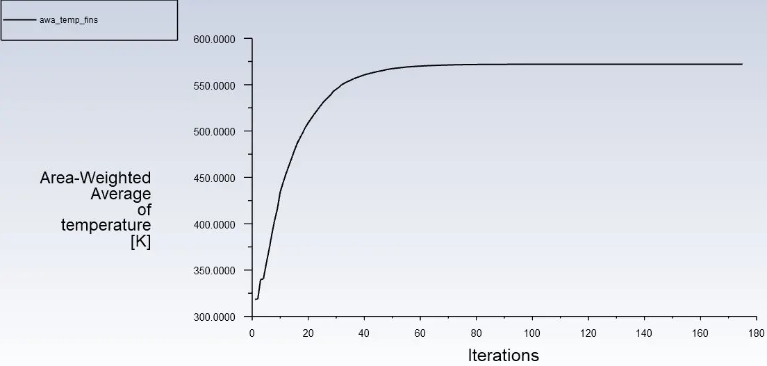
Fig 34: Temperature at Fins
4. Area Weighted Average of Surface Heat Transfer Coefficient at Processor = 6.64 W/m^2 K
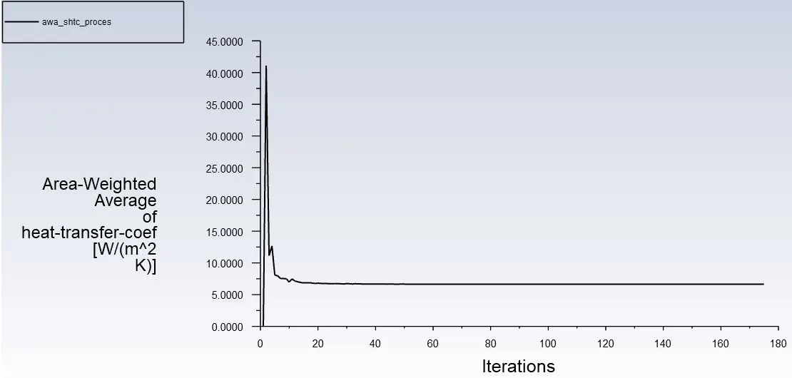
Fig 35: Surface Heat Transfer Coefficient at Processor
5. Area Weighted Average of Surface Heat Transfer Coefficient at Fins = 19.62 W/m^2 K
Fig 36: Surface Heat Transfer Coefficient at Fins
6. Contours of Temperature
Fig 36: Temperature contours for V = 1 m/s
Here we can see how heat is getting dissipiated in the direction of flow.
7. Contours of Velocity
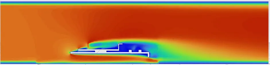
Fig 37: Velocity Contours for V= 1m/s
We can see that this graphic card is a typical case of bluff body, the wake region does indicate saperated flow. The flow in the wake is turbulent and rate of heat transfer will also increase in the wake as can be confirmed from the temperature contours.
8. Heat Dissipiation through Base of Graphics Card
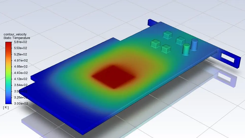
Fig 38: Temperature Hot spots for V=1m/s
As thermal conductivity of base material is low (FR4), a temperature hotspot can be observed in the vicinity of the processor.
Case 2: V = 3 m/s
1. Residuals
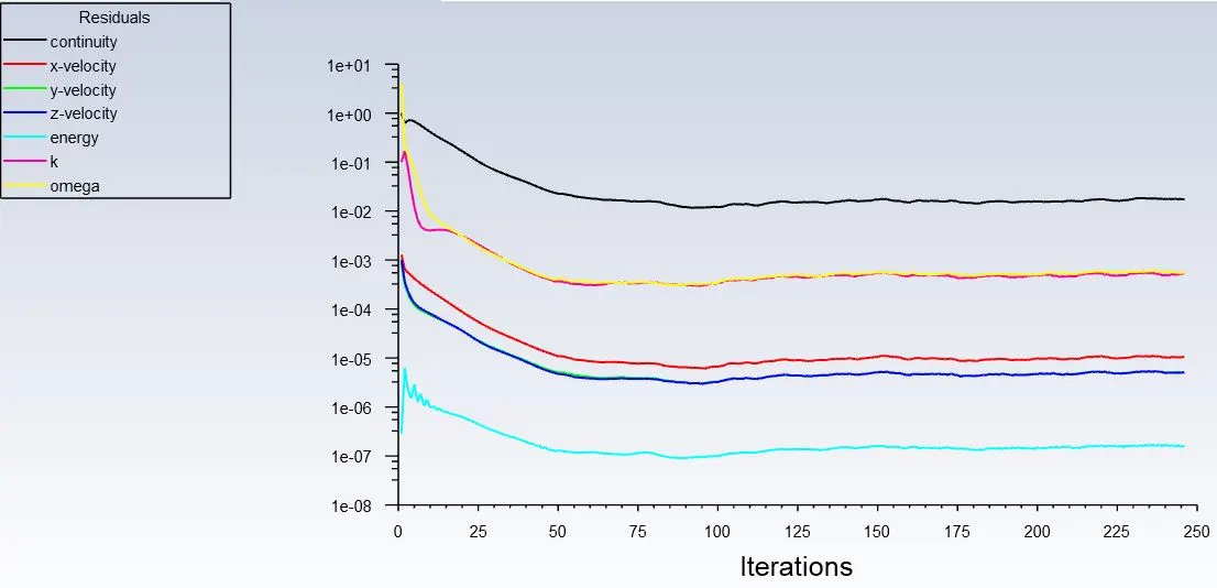
Fig 39: Residuals for V = 3m/s
As velocity increases, flow gets even more Turbulent and Continuity residuals are even harder to Converge. There are two ways to counter this issue, we can improve the mesh Quality or we can reduce the under-relaxation factors.
Default Under-Relaxation Factors
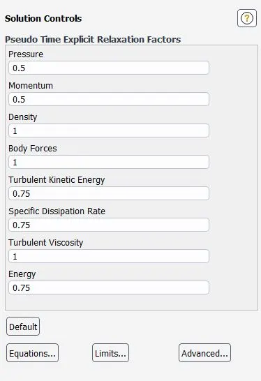
Fig 40:
Reducing Under-Relaxation Factors
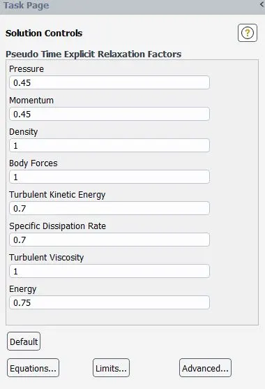
Fig 41:
Improved Residuals
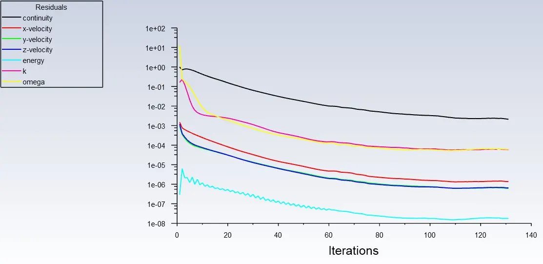
Fig 42: Residuals for case 2
We can see clearly that residuals are not diverging now. This shows how relaxation factors can impact the convergence of a solution.
2. Area Weighted Average of Temperature at Processor = 440.18 K
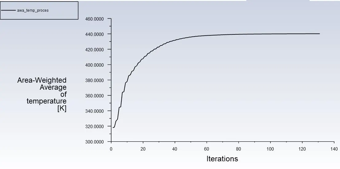
Fig 42: Temperature at Processor for Case 2
3. Aerea Weighted Average of Temperature at Fins = 434.02 K
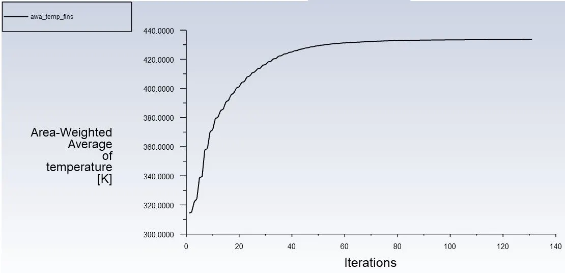
Fig 43: Temperature at Fins for Case 2
4. Area Weighted Average of Surface Heat Transfer Coefficient at Processor = 12.80 W/m^2 K
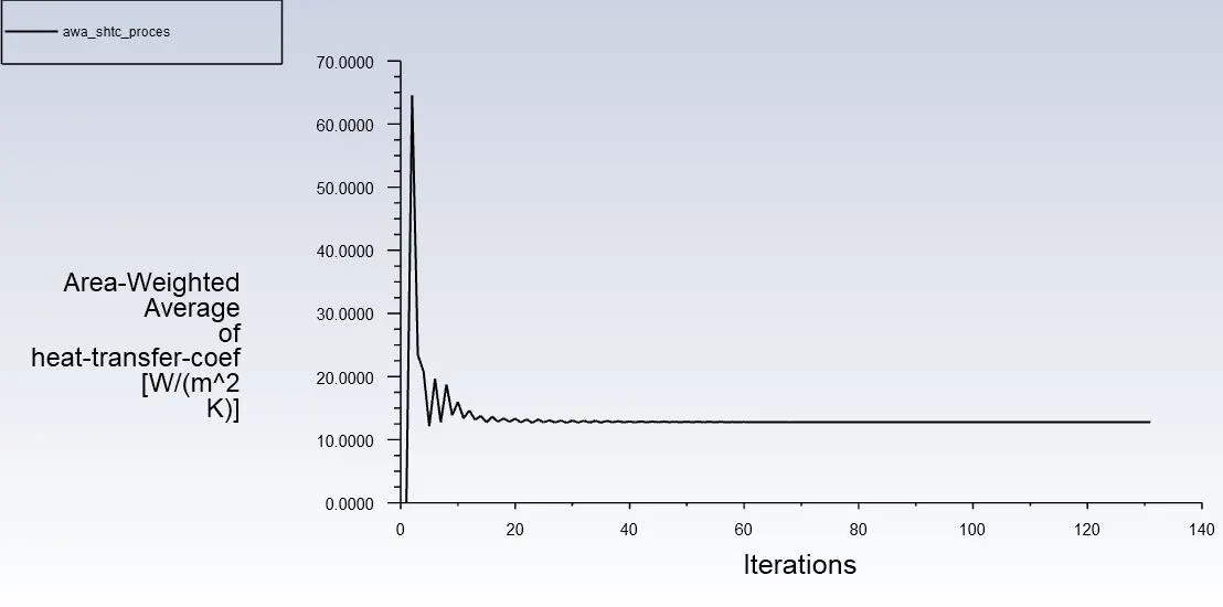
Fig 44: Surface Heat Transfer Coefficient For Case 2
5. Area Weighted Average of Surface Heat Transfer Coefficient at Fins = 38.86 W/m^2 K
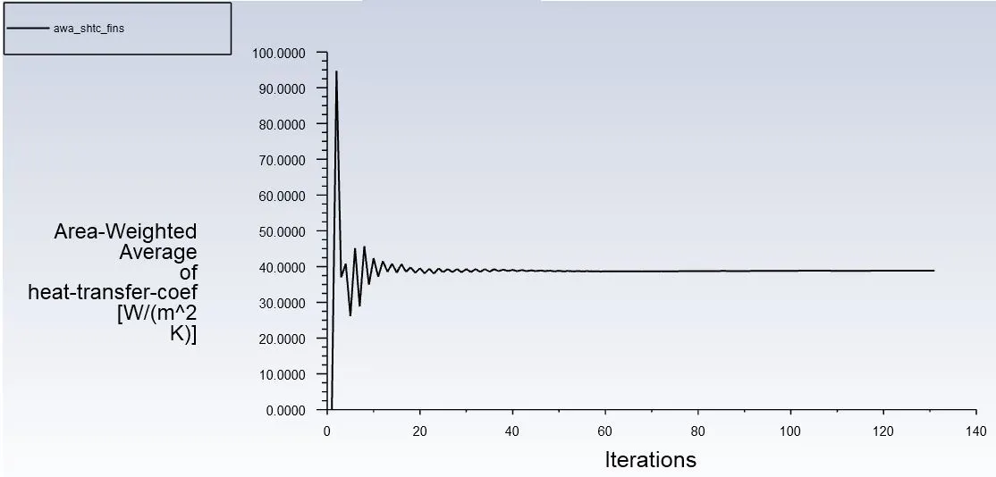
Fig 45: Surface Heat Transfer Coefficient for fins case2
6. Contours of Temperature
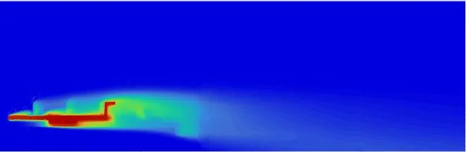
Fig 46: Temperature Contours for Velocity = 3m/s
7. Contours of Velocity
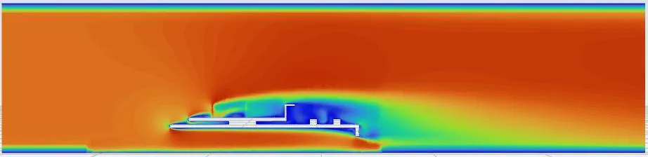
Fig 47: Velocity Contours for V = 3m/s
8. Heat Dissipiation through Base of Graphics Card
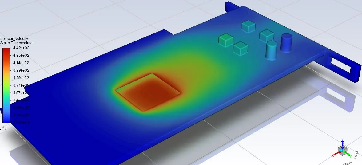
Fig 48: Temperature Hotspots for V = 3m/s
Case 3: V = 5m/s
1. Residuals
Fig: 49 Residuals for Case 3
Once again we see that under default under-relaxation factors, the residuals are not converging.
Reducing Under-Relaxation Factors
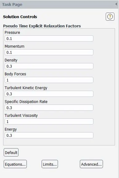
Fig 50: Changed Relaxation Factors
Improved Residuals
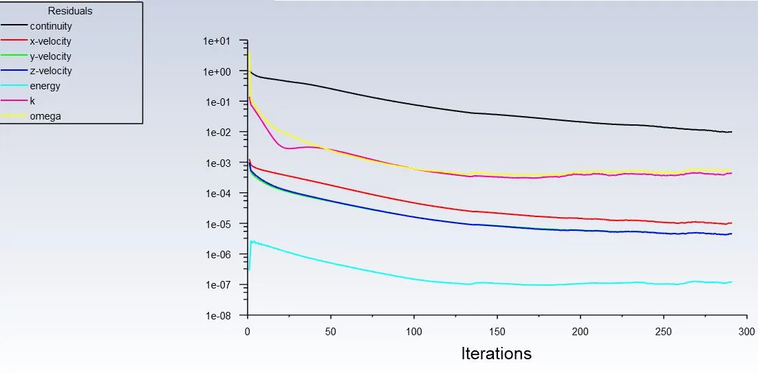
Fig 51: Residuals for Cse 3 Improved
2. Area Weighted Average of Temperature at Processor = 402.06 K
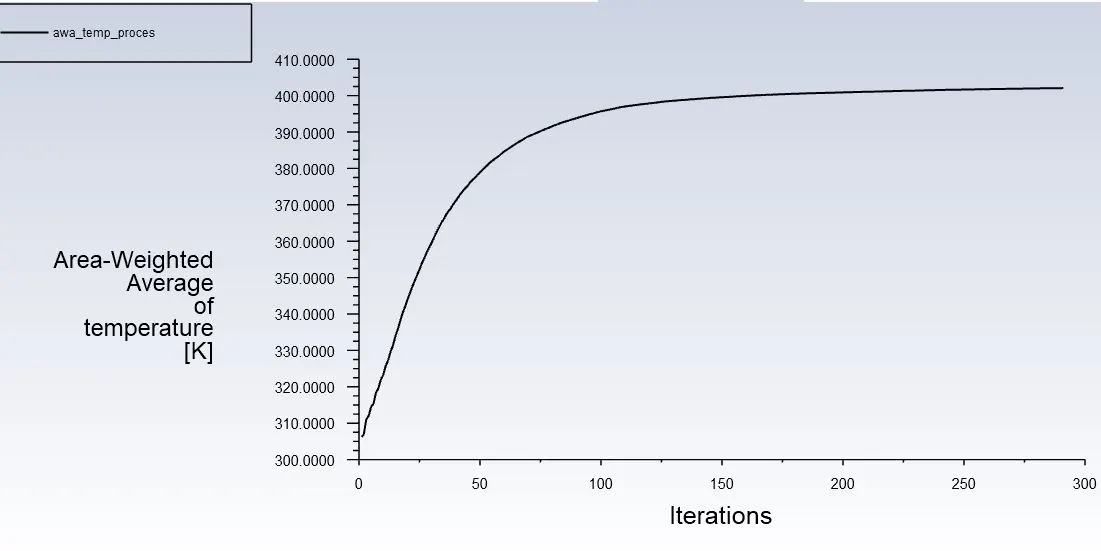
Fig 52: Temperature at Processor Case 3
3. Aerea Weighted Average of Temperature at Fins = 395.47 K
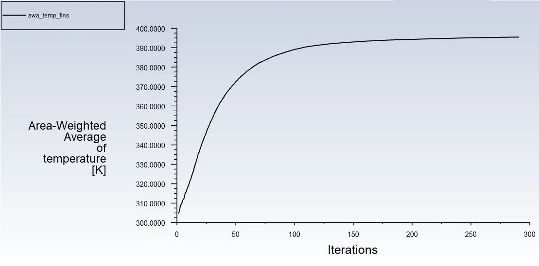
Fig 53: Temperature at fins Case 3
4. Area Weighted Average of Surface Heat Transfer Coefficient at Processor = 20.46 W/m^2 K
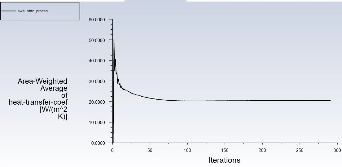
Fig 54: Surface Heat Transfer Coefficient for Processor case 3
5. Area Weighted Average of Surface Heat Transfer Coefficient at Fins = 52.75 W/m^2 K
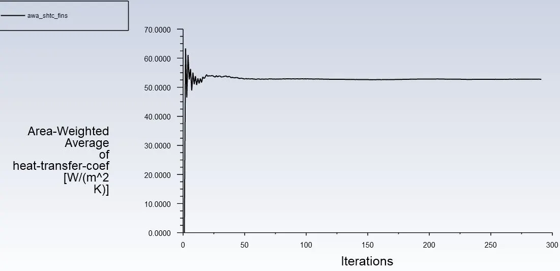
Fig 55: Surface Heat Transfer Coefficient for fins case 3
6. Contours of Temperature
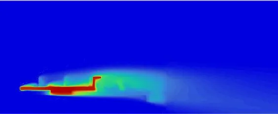
Fig 56: Temperature Contours for Case 3
7. Contours of Velocity
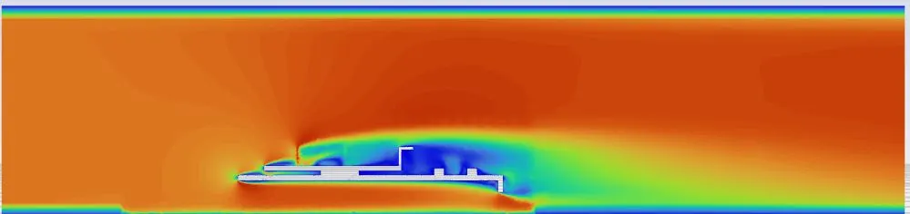
Fig 57: Velocity Contours for V = 5 m/s
8. Heat Dissipiation through Base of Graphics Card
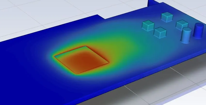
Fig 58: Temperature Hotspots for V = 5m/s
Summary of Results-Numerical
| Case | Velocity [m/s] | Awa of Temperature at processor [K] | Awa of Temperature at fins [K] | Awa of Surface Heat Transfer Coefficient at Processor [W/m^2K] | Awa of Surface Heat Transfer Coefficient at Fins [W/m^2K] |
| 1 | 1 | 578.74 | 572.07 | 6.64 | 19.62 |
| 2 | 3 | 440.18 | 434.02 | 12.80 | 38.86 |
| 3 | 5 | 402.06 | 395.47 | 20.46 | 52.75 |
Table 2: Summary for all Cases
Summary of Results-Graphical
1. Velocity Vs Surface Heat Transfer Coefficient at Fins
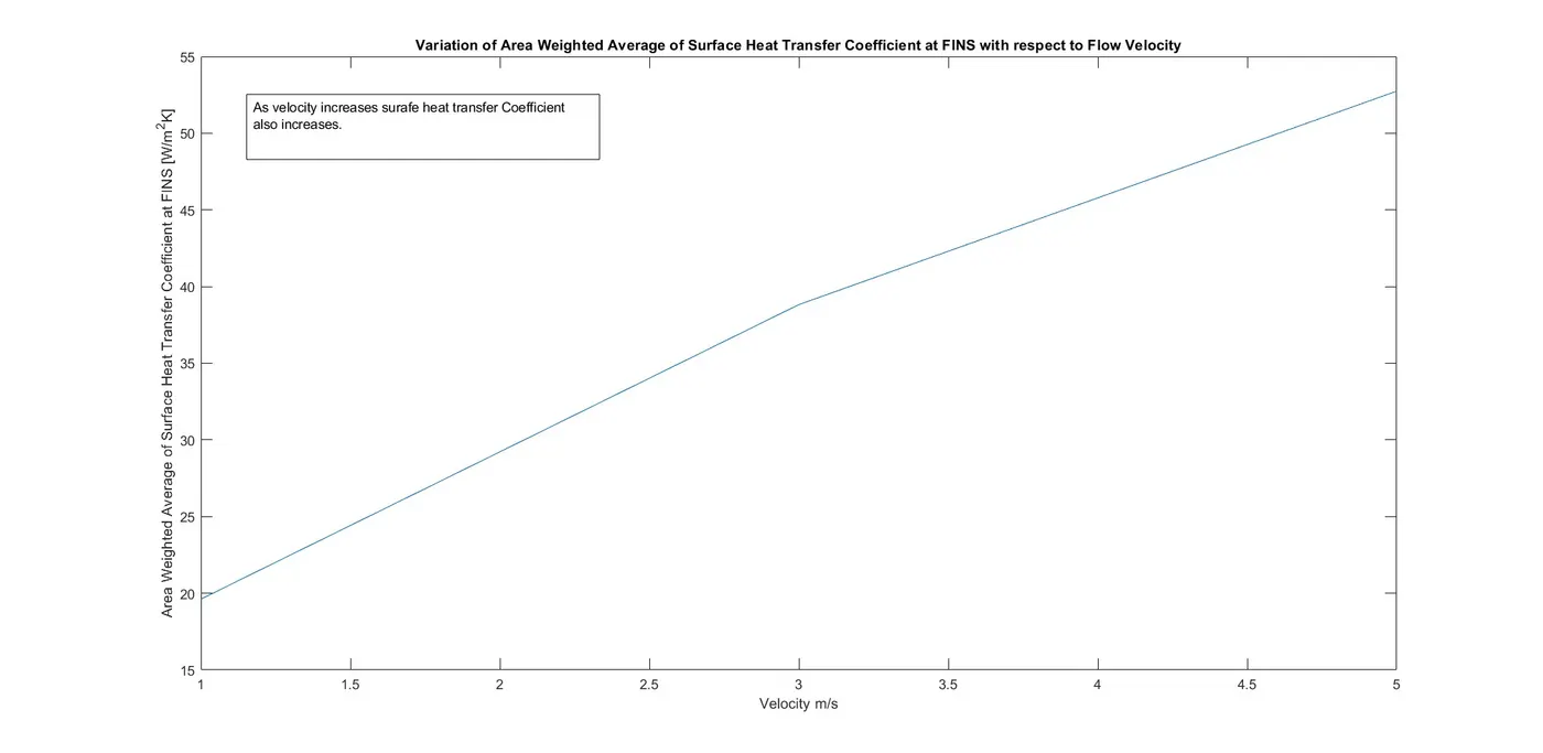
Fig 59: SHTC at fins vs Velocity
2. Velocity Vs Surface Heat Transfer Coefficient at Processor
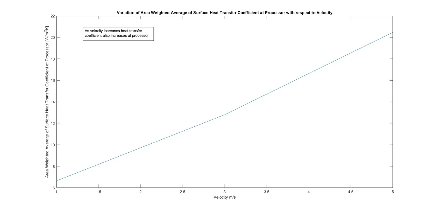
Fig 60: Shtc at processor Vs Velocity
3. Velocity Vs Temperature at Fins
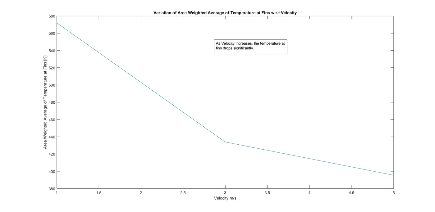
Fig 61: Temperature at Fins Vs Velocity
4. Velocity Vs Temperature at Processor
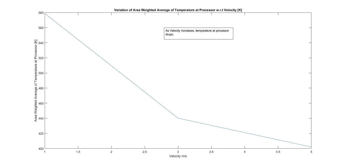
Fig 62: Temperature at Processor Vs Velociy
Observation:
Reflecting from Newton's Law of Cooling;
The rate of heat flux between a flowing fluid and stationary solid is given by,
d/dt (q/A) ∝ (T(fluid) - T(solid))
= -h*A*(T(fluid) - T(solid))
where, h is constant of proportionality called convection heat transfet coefficient. [w/m^2 K]
h = f(thermophysical properties of the fluid, velocity of the fluid)
=> if anywhere in the computational domain velocity increases, the heat transfer coefficient must also increase.
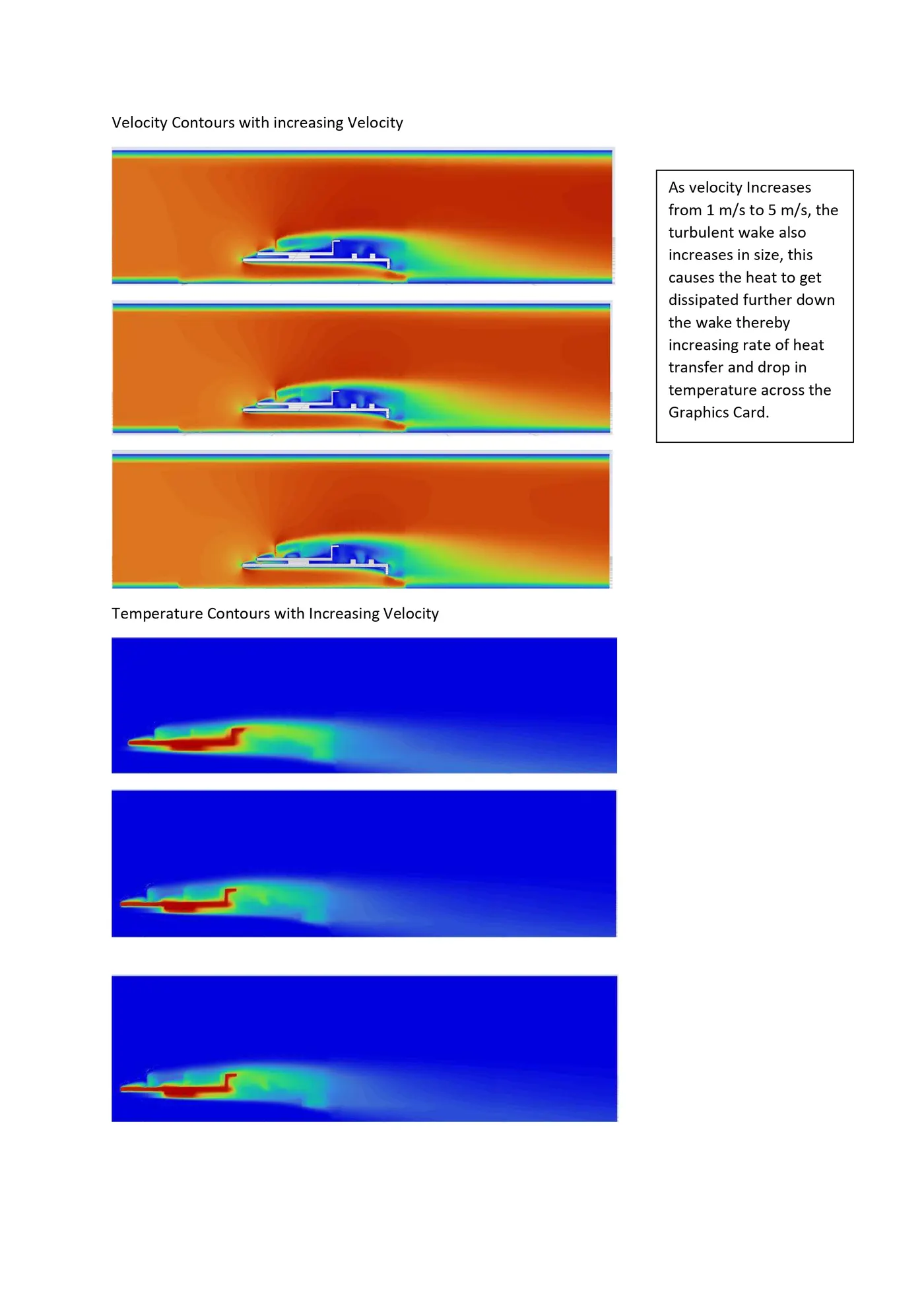
Thus we can deduce two conclusions from our Numerical Data presented Graphically:
1. As velocity increases, the surface Heat Transfer Coefficient also increases and thus rate of heat transfer increases.
2. As heat is getting dissipiated, thus due t rate of heat transfer increasing due to increase in velocity, the temperature of Graphic Card also decreases.
Graphically Demonstrating the Observations
Conclusions
1. The fundamental physics of Conjugate Heat Transfer is pivotal in managing the Heat Loads of a Graphics Card.
2. The rate of Heat Transfer can be increased by increasing the Surface Heat Transfer Coefficient.
3. The Surface Heat Transfer Coefficient increases with velocity, so higher velocity of air means better cooling of Graphics Card.
4. As rate of Heat Transfer Increases, the temperature of Graphics Cards drops.
5. With increasing velocity the temperature of graphics card will keep droping.