Week 7 Challenge

Week 7

1) Simulink model for a vehicle model

Aim:

To create the vehicle model by considering forces acting on vehicle and vehicle dynamics with velocity as output.

Software used:

• MATLAB/ Simulink

Blocks used:

• Constant
• Integrator
• Differentiator
• Product
• Add
• Saturation
• Terminator
• Inport
• Outport
• Goto
• From
• To workspace

Model:

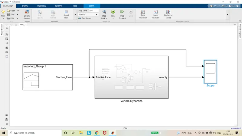
Vehicle Dynamics Subsystem:

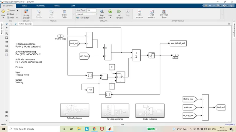
Explanation:

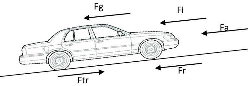
Whenever the vehicle moves on the road, various forces acts on the vehicle. The forces are

1. Traction force
2. Rolling resistance force
3. Air drag resistance force
4. Hill climbing force

Traction force:

This force is used to move the vehicle forward. This force is given by the powertrain of the vehicle. This force is opposed by the other forces. This is the only aiding force of the vehicle.

Rolling resistance force:

Rolling resistance force is the force due to the friction of tyre and surface. Factors that contribute to rolling resistance are deformation of the wheels, the deformation of the roadbed surface, and movement below the surface Rolling resistance force can be formulated by multiplying the weight of the vehicle and coefficient of rolling resistance. Weight of the vehicle is m*g. Coefficient of rolling resistance varies according to the various surfaces such as asphalt, concrete, tar, soft soil, liquid, icy roads, mud, etc.

Rolling resistance force = U_res*Veh_mass*g*cos(alpha)

U_res = Coefficient of rolling resistance = 0.015

Veh_mass = Mass of the vehicle = 1500 kg

g = gravity = 9.8 m/s

alpha = angle in radians

This formula is designed in Simulink.

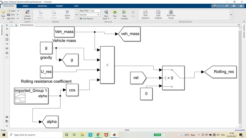
Rolling resistance occurs only while running. i.e., the velocity v ~= 0. If the velocity is equal to zero then rolling resistance equal to zero. This can be done with help of switch.

Air drag force:

Air Drag force is the force due to wind velocity opposing the vehicle on the frontal area. Air drag force on the vehicle is minimum when the vehicle is moving slowly. If the speed increases, the air drag force also increases. It is due to during low speed the pressure in the front and back side of the vehicle is more or less same. If the speed is high, the pressure in the front of the vehicle is higher than the rear side of the vehicle. This creates the opposing force on the vehicle. Air drag force can be identified by using the above formula. this varies with the square of the speed.

Air drag force = (1/2)*Cd*Af* delta*V^2

Cd = Drag coefficient = 0.3

Af = Frontal area = 2 m^2

Delta = Air density = 1.225 kg/m^3

V = Velocity of vehicle in m/s

This is formulated in simulink.

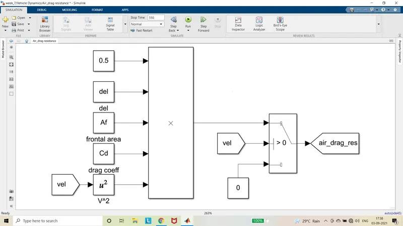
Same like rolling resistance, Air drag resistance occurs only while running. i.e., the velocity v ~= 0. If the velocity is equal to zero then air drag resistance equal to zero. This can be done with help of switch.

Hill climbing force:

Hill climbing force (grade resistance) is the force acting against the direction of acceleration of vehicle when the vehicle moving at a certain angle (slope). This force is acting in opposite due to gravity.

Hill climbing force=Veh_mass*g*U_res*sin (alpha)

U_res = Coefficient of rolling resistance = 0.015

Veh_mass = Mass of the vehicle = 1500 kg

g = gravity = 9.8 m/s

alpha = angle in radians

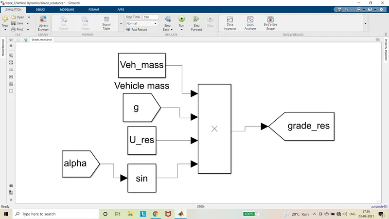
Parameters:

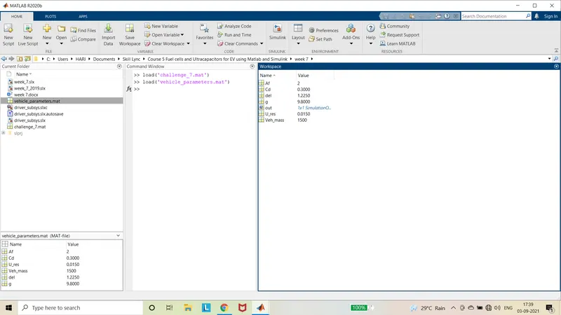
Procedure:

• The summation of rolling resistance force, air drag resistance force and grade resistance is the total opposing force.
• This opposing force is subtracted from the tractive force which gives the resultant force to move the vehicle.
• The tractive force must be higher than the opposing force to move the vehicle.
• The tractive force is given by the powertrain block.
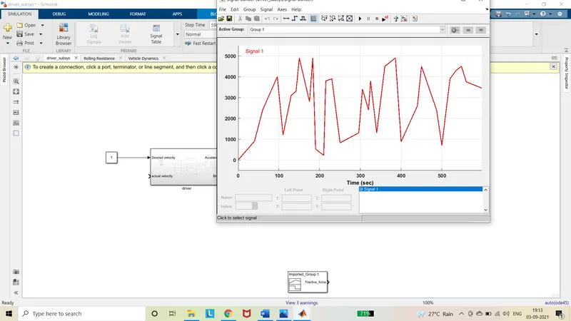
• Here we can give the custom force (assumed) directly by using the signal builder block.
• The slope of the road is also given by using the signal builder block which is loaded from the .mat file.
• The parameters are loaded from .mat to MATLAB.
• The output we want is the velocity.
• So, this force is divided with vehicle mass to get the acceleration.
• This acceleration is then integrated to get the velocity.
• But due to the integral windup the overshoot occurs.
• This occurs because initially the error between the actual and desired velocity is more. In order to overcome this error, the overshoot occurs.
• Then due to this overshoot, another fluctuation less than desired velocity to overcome the error due to overshoot.
• This windup can be overcome by using anti windup. This is obtained by using external reset.
• When the acceleration and velocity is not equal to zero, then external reset is set.
• When the acceleration and velocity is zero, then the external reset is reset.
• By considering the initial condition of vehicle which is zero, in order to reject the unwanted errors, the memory is used.
• Then the saturation block is used to get the forward velocity from zero to infinity.
• This gives the output velocity of the vehicle.

Alpha values:

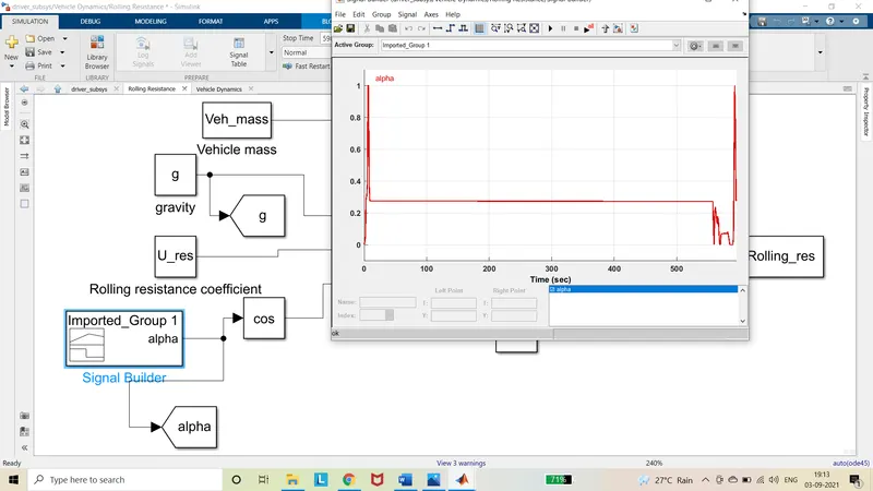
Input force:

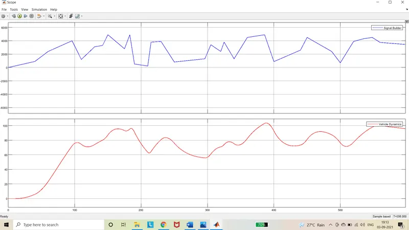
Output scope:

Output velocity:

Summary:

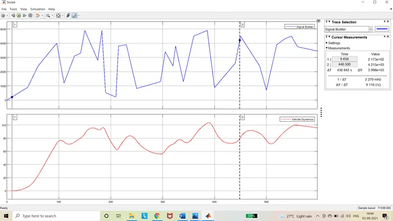
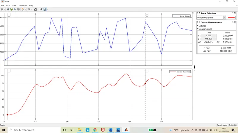
From the above plot it is clearly observed that when the force on the vehicle increases, the velocity of the vehicle increases. If the velocity of the vehicle decreases, the velocity of vehicle decreases. In addition to that if the second and third plot is observed in the cursor measurements, when the force is increased to particular value but the velocity of the vehicle is zero. This indicates, that particular force is equal to the opposing force of the vehicle for the given parameters. In this model the force at 9.65 seconds is 217.3Nm but the velocity is perfect zero. It shows that the opposing force of the vehicle is 217.3Nm for given parameters.