Week 7 - Auto ignition using Cantera

AIM: To perform Auto Ignition using Cantera

Part 1:

Performing Simulation on Auto-Ignition and Ignition delay on Methane on variation temperature and pressure with a simulation time of 10secs in below two cases

• Case:1 Plotting the variation of Auto Ignition time of Methane with a constant temperature of 1250K and pressure varying from 1 to 5 atm.
• Case:2 Plotting the variation of Auto Ignition time of Methane with a constant pressure of 5 atm and temperature varying from 950K to 1450K.

Part 2:

To Calculate and illustrate the rate of change of molar concentrations of the given elements "H2O, O2, OH" with respect to the time at simulation time = 10 secs in the below two cases

• Case :1 When the Temperature is 1000K and the pressure 5 bar
• Case:2 When the Temperature is 500K and the pressure 5 bar

Auto-Ignition:

The fuel particles auto-ignite. This normally happens after the spark has been introduced. Auto-Ignition depends upon the Self-ignition temperature, fuel-air mixture ratio, Value timings, angle of spark plug and initial temperature of the cylinder.

Basically, when we have a high cylinder temperature, the fuel particles are almost near to their combustion temperature. So, when the spark is introduced, the flame front propagates, this flame boundary further increases the temperature of the fuel molecule, which is already at a high temperature. Keep in mind that the flame has not reached the molecule yet. This high pressure and temperature of the molecule, allows itself to be oxidized (Burn). So, this molecule would have a separate flame in front of its own, let's call it local flame front. When the main flame front and the local flame front, collide, we have a jerk inside the Engine. This is what we call knocking.

Ignition Delay:

The time interval between the start of injection and the start of combustion. This delay period consists of (a) physical delay, wherein atomization, vaporization, and mixing of air-fuel occur, and (b) chemical delay attributed to pre-combustion reactions. Physical and chemical delays occur simultaneously. To reduce NOx, the method adopted in modern engines is to reduce the ignition delay.

For predicting heat release in modern engines, therefore, the estimation of ignition delay is no more important. However, the ceiling on NOx is dipping to such a low level that accurate prediction of ignition delay has become important even if it is small.

Calculating Ignition Delay:

TimeignitionDelay=IntialTemperature+400K

Solution:

Part 1:

In this part, we are going to simulate the Auto Ignition Time for Methane under the following conditions, of varying temperature and pressure parameters using the Cantera module in python.

Case 1:

Plotting the variation of Auto Ignition time of Methane with a constant temperature of 1250K and pressure varying from 1 to 5 atm.

Python Code:

'''
	Calculating Ignition Delay Using Reactor and ReactorNet Using Cantera
'''
import sys
import cantera as ct
import matplotlib.pyplot as plt
import numpy as np

gas = ct.Solution('gri30.xml')
p_start = ct.one_atm
p_end = ct.one_atm*5
n = 5
pressure = np.linspace(p_start,p_end,n) # pressure Variation
ignition_delay=[]

for i in range(1,6):

	P=ct.one_atm*i # pressure variation from 1 atm to 5 atm.
	T=1250 # Temperature
	gas.TPX=T,P,{'CH4':1,'O2':2,'N2':7.52}
	r=ct.IdealGasReactor(gas)
	sim=ct.ReactorNet([r])
	time=0
	sim_time=10*100
	states=ct.SolutionArray(gas,extra=['time_in_ms','t'])
	T_old=T

	# Time loop
	for j in range(sim_time+1):
		time+=1e-3
		sim.advance(time) # Time step
		states.append(r.thermo.state,time_in_ms=time*1e-3,t=time)	

		T_new = states.T
		T_new = T_new[j-1]

		if (T_new-T_old)>=400:
			ignition_delay.append(time)

		T_old = states.T
		T_old = T_old[j-1]

		#ploting
	plt.subplot(2,1,1)
	plt.plot(states.t,states.T)
	plt.xlabel('Simulation time (ms)')
	plt.ylabel('Temprature(k)')
	plt.legend(['Pressure -'+str(P)+'[atm]'for P in pressure])

plt.subplot(2,1,2)
plt.plot((pressure/101325),ignition_delay,'-o')
plt.xlabel('Pressure')
plt.ylabel('ignition_delay')	
plt.show()

Result:

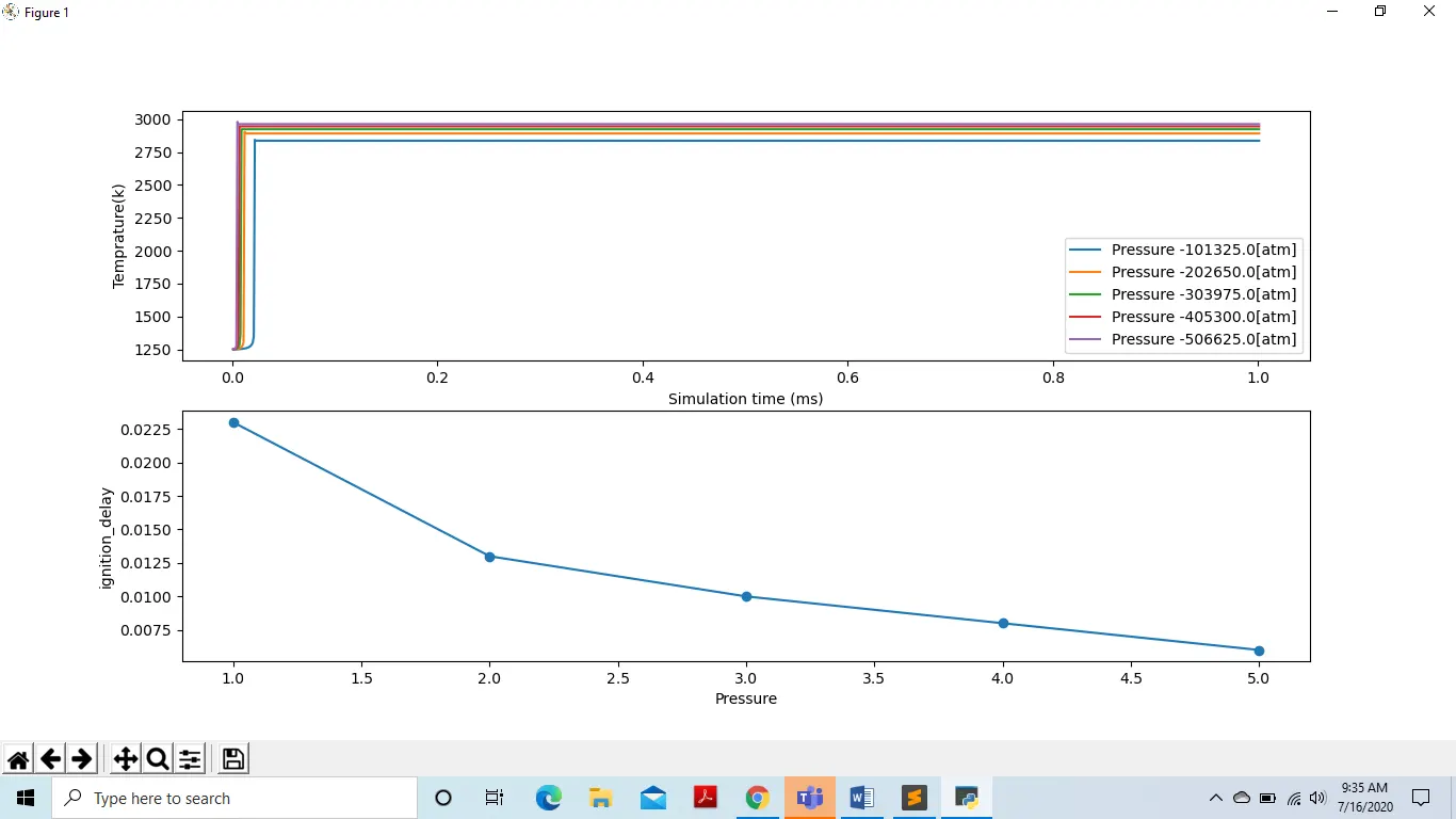
Below we can see the plot of Methane under the variation of Pressure and Temperature, The above plot given the Variation of pressure given time, Observing the plot The pressure increases, as well as temperature increases, At initial pressure needs more time to Auto-Ignite and produce low temperature.

The second Plot defines Ignition-delay, we can see that if pressure increases ignition delay decreases, Why? According to Ideal gas, equation pressure is directly proportional to the temperature and Initial temperature is high ignition delay is low.

Case 2:

In this case, Plotting the variation of Auto Ignition time of Methane with a constant pressure of 5 atm and temperature varying from 950K to 1450K.

Python code:

'''
	Calculating Ignition Delay at constant pressure and Variation Temperature
'''
import sys
import cantera as ct
import matplotlib.pyplot as plt
import numpy as np

gas = ct.Solution('gri30.xml')
T_start=950 # intial temperature
T_end=1450 # final temperature
n=10
Temp=np.linspace(T_start,T_end,n)
ignition_delay=[]

for i in range(len(Temp)):

	P=ct.one_atm*5 # Constant pressure
	gas.TPX=Temp[i],P,{'CH4':1,'O2':2,'N2':7.52}
	r=ct.IdealGasReactor(gas)
	sim=ct.ReactorNet([r])
	time=0
	states=ct.SolutionArray(gas,extra=['time_in_ms','t'])
	sim_time=10*100
	T_old = Temp[i]

	#Time loop
	for j in range (sim_time+1):
		time+=1e-3
		sim.advance(time)
		states.append(r.thermo.state,time_in_ms = 1e-3*time, t= time)

		# calculating ignition delay
		T_new = states.T
		T_new = T_new[j-1]

		if ((T_new-T_old)>=400):
			ignition_delay.append(time)

		T_old = states.T
		T_old = T_old[j-1]

	# Ploting
	plt.subplot(2,1,1)
	plt.plot(states.t,states.T)
plt.xlabel('Simulation time(ms)')
plt.ylabel('Temperature(k)')
plt.legend(['Intial_T ='+str(T) +'[k]' for T in Temp])

plt.subplot(2,1,2)
plt.plot(Temp,ignition_delay,'-o')
plt.xlabel('Intial temperature (k)')
plt.ylabel('ignition_delay')
plt.show()

Result:

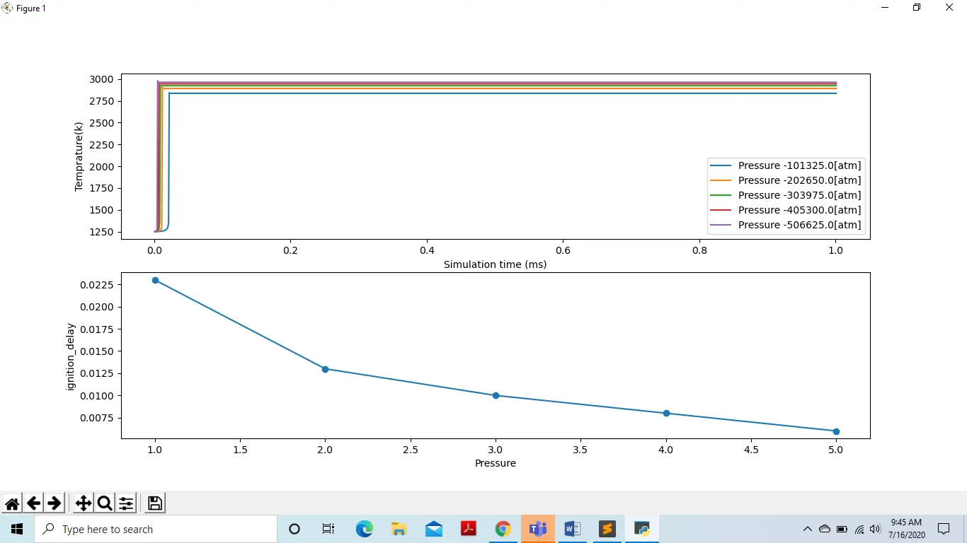
Below we can see the plot of Methane under the variation of temperature and constant pressure, The above plot gave the Variation of temperature given time.

Observing the plot The Temperature increases, as well as ignition delay decreases. At initial temperature needs more time to Auto-Ignite. As we can see below the graph, if the temperature is low, the ignition delay high, and the initial temperature is high ignition delay is low. As compared to the pressure the ignition delay is faster because of the temperature high. It may help with the auto-ignition.

Part 2:

In this case Further, observe and print the rate of change of molar concentrations of the given elements "H2O, O2, OH" with respect to the time, (simulation time = 10 secs) at 2 different Cases

• When Temperature is 1000K and the pressure 5 bar
• When Temperature is 500K and the pressure 5 bar

CH4 + 2(O2 + 7.52N2) = CO2 + 2H2O + 7.52N2

In this case, we are Calculating the molar fraction of product species using Cantera in the python module.

Python code:

'''
	Calculating Rate of change of concentration of species H2O,O2,OH
'''
import numpy as np
import cantera as ct
import sys
import matplotlib.pyplot as plt

Temp = [1000,500]

for T in Temp:
	gas = ct.Solution('gri30.xml')
	P = ct.one_atm*5
	gas.TPX = T,P,{'CH4':1,'O2':2,'N2':7.52}
	r = ct.IdealGasReactor(gas)
	sim = ct.ReactorNet([r])
	time = 0
	states = ct.SolutionArray(gas,extra=['time_in_ms','t'])
	sim_time = 10*100
	for i in range(sim_time+1):
		time+=1e-3
		sim.advance(time)
		states.append(r.thermo.state,time_in_ms=time*1e-3,t=time)

	# Plot Rate of H2O Molarfraction
	plt.subplot(1,3,1)
	plt.plot(states.t,states.X[:,gas.species_index('H2O')])
	plt.xlabel('Simulation time')
	plt.legend(['H2O-Molefraction'])
	plt.title('Rate of concentration of H2O')

	
	# Plot Rate of O2 Molarfraction
	plt.subplot(1,3,2)
	plt.plot(states.t,states.X[:,gas.species_index('O2')])
	plt.xlabel('Simulation time')
	plt.legend(['O2-Molefraction'])
	plt.title('Rate of concentration of O2')


	# Plot Rate of OH Molarfraction
	plt.subplot(1,3,3)
	plt.plot(states.t,states.X[:,gas.species_index('OH')])
	plt.xlabel('Simulation time')
	plt.legend(['OH-Molefraction'])
	plt.title('Rate of concentration of OH')
	plt.suptitle('Rate of change of concentration of H20 ,O2 and N2 at' + str(T) + '[Kelvin]')
	plt.show()
	

Result:

Case:1

When Temperature is 1000K and the pressure 5 bar

In this case, Calculate the molar fraction of products species using Cantera

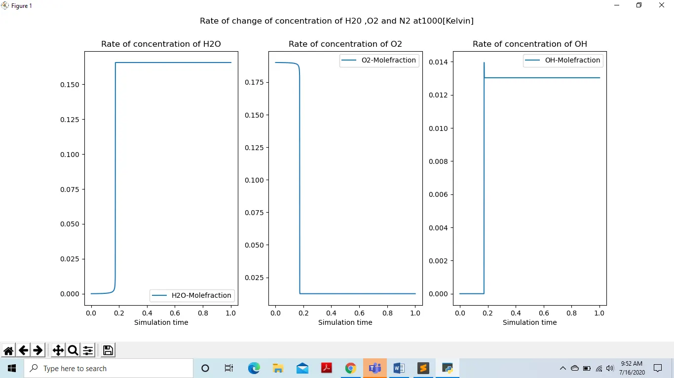
In the below figure, we can see the rate of the molar fraction of H2O, O2, and OH at 1000K.

The first plot tells the mole fraction of H2O it is respectively very less before auto-ignition. As we discussed before The Reaction of Methane and Air its forms the product of H2O and its starts very less after ignition takes place it becomes increases and somewhere it gets to stability this is called equilibrium chemistry.

The second plot is to define the mole fraction of O2 its respectively decreases because it is air and reacts with fuel and gets oxidized.

The third plot tells the mole fraction of OH it is respectively very less before auto-ignition. As we discussed before The Reaction of Methane and Air its forms the product of OH and its starts very less after ignition takes place it becomes increases and somewhere it gets to stability this is called equilibrium chemistry.

Case:2

When Temperature is 500K and the pressure 5 bar

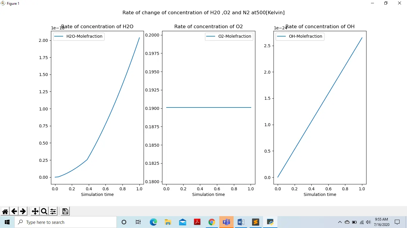
In this case, the calculated molar fraction of H2O, O2, and OH is at 500k. the rate mole fraction is very less as compared to the 1000K because the initial temperature was very low. In the first plot we see that very slowly Auto-ignition takes place and the second plot O2 is not completely automized because the initial temperature was very low.