Week 7 - Simulation of a 1D Super-sonic nozzle flow simulation using Macormack Method

Objective

• To write the code for both conservative and non-conservative forms of governing equations which is solving the 1D supersonic nozzle flow equation using the Maccormack Method.
• Determining the minimum number of cycles in which the solution gets converged under both the scenarios and comparing the mass flow rates under 2 conditions.
• Determining the fastest process among the 2 processes and performing the Grid dependence test.

Let's get Intro

Usually, a numerical solution of the steady, isentropic quasi 1D nozzle flow is redundant because the analytical solution for this
the problem already exists but the main aim here is to find the solutions for the above flow problem numerically by applying the
various CFD techniques which can be supporting evidence for the analytical solution.

Flow which is considered here is the steady, isentropic flow through a convergent-divergent nozzle. The flow at the inlet to the
nozzle comes from a reservoir where the pressure and temperature are denoted by p0 and T0 respectively. The cross-sectional
area of the reservoir is large and hence the velocity is very small.

The flow is locally subsonic in the convergent section of the nozzle, at the throat section the flow is sonic and then as the area
of the nozzle increases, the flow gets converted into supersonic at the divergent section.

Normally in reality flow properties vary in both x and y directions, but here in this project, we make the assumption that the flow properties vary only along the x-direction. So, the flow under the assumption is called Quasis dimensional Flow.

Here the problem is solved with a time-marching solution using Maccormack Method

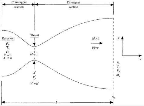
Figure (a): Schematic of the subsonic nozzle

MacCormack's Techniques

MacCormack's Techniques is the explicit finite difference technique that is second-order accurate in both space and time. This method is very effective where we can obtain second-order accuracy with first-order terms and the mathematical complexity of calculating the second-order time derivative can be avoided.

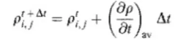
In this method variable at grid point (i,j) at time t+dt is calculated by using

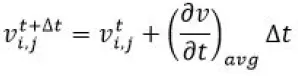
Here in this time marching is split into two steps i.e predictor and corrected step.

1. Initially, we start with initial conditions.
With the help of initial conditions, we calculate the predictor step.

In this step, the spatial derivatives on the right side are replaced with forward differences.

`(∂ρ/∂x)predictor=(ρ(i+1)-ρ(i))/dx`

With the predicted value of the time derivative, we determine the value of 'F' which is called the solution update step.
Now, these values of the update step are used in the corrected step.

Corrected step

In the corrected step the spatial derivatives on the right side are replaced with a backward difference.
considering the example of density

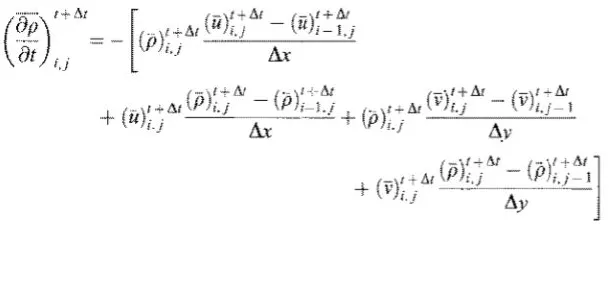
Now once after calculating the corrected step, a new time derivative is calculated with the help of both predicted and corrected time derivatives.

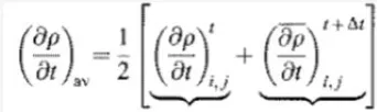
Once calculating the average value, the final solution is obtained with the help of average time derivatives

Governing Equations for 1D Quasi supersonic nozzle flow

Governing equations are of two types
1.Conservative form.
2.Non-Conservative form.

Non-conservative form of equations
Continuity:

Momentum:

Energy:

All the above equations consist of non-dimensional variables

Calculation of Time Step

In this solution magnitude of the time step is calculated based on the Courant number(C). The simple stability analysis of linear hyperbola equations gives that any value of C less than 1 gives a stable solution.

for this problem value of C is considered as 0.5.

The magnitude of dt is calculated by using the formula is

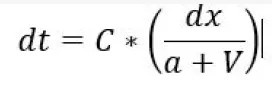
With the help of the above formula, the value of dt is calculated at each node. Once after calculating the dt value at all the nodes minimum of all dt is considered.

Boundary Conditions

At the inlet, the flow variables such as temperature and density remain constant and the value of velocity changes.

v1=2*v2-v3

At outlet conditions, all the flow variables keep on changing

Vn=2*Vn-1 - Vn-2

(Rho)n=2*(Rho)n-1 - (Rho)n-2

Tn=2*Tn-1 - Tn-2

Initial Conditions

Area A = 1 + 2.2*(x-1.5)^2
Density rho=1-(0.3146*x)
Temperature T=1-(0.2314*x)
Velocity v=(0.1+(1.09*x)).*(T.^0.5)

Conservative form of equations

The equations for Quasis 1D flow are expressed in the generic form. The equations consist of Solution vector U and the flux vector F and the Source term J as follows.

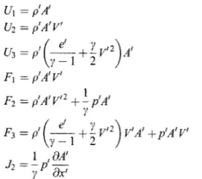
With the help of the above elements, solution vector equations can be written as

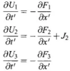
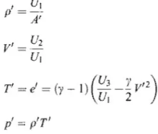
Once after solving the above equations our numerical solution will give the results for the solution vector U (U1, U2, U3) in steps of time, this the reason why U is called as Solution vector. In order to obtain the primitive variables density, Velocity,
Temperature and pressure Solutions vector must be decoded.

Boundary Conditions

At Inlet boundary conditions the value U1 stays fixed and other two solution vector U2 and U3 will float with respect to time

U2=2*U2-U3;

U3= U1*((T/(gamma-1))+((gamma/2)*(v^2)))

At Outlet boundary conditions the values of solution vector of U1,U2 and U3 will be changing with respect to time.

U1(n)=(2*U1(n-1)-U1(n-2))
U2(n)=(2*U2(n-1)-U2(n-2))
U3(n)=(2*U3(n-1)-U3(n-2))

Intial conditions

Area A = 1 + 2.2*(x-1.5)^2 it remains constant throughout the nozzle.

Velocity= 0.59/(rho*A)

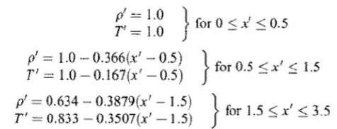
At t=0, values of density and temperature throughout the nozzle are given as follows

Procedure

Let's Code for the Non-Conservative form of the equation

%solving quasis 1D supersonic nozzle flow using maccormack method for nonconservative eq
clear all
close all
clc
%inputs
n=31;
x=linspace(0,3,n);
dx=x(2)-x(1);
gamma=1.4;
%calculate intial profiles
rho=1-(0.3146*x);
T=1-(0.2314*x);
v=(0.1+(1.09*x)).*(T.^0.5);
a=1+(2.2*((x-1.5).^2));
%courant number
c=0.5;
%finding the throat grid point
thr=find(a==1);
%for loop to determine the dt values at each value
for m=1:n
dt_grid(m)= c*(dx/((T(m))^0.5 + v(m)));
end
%determimg the dt value
dt=min(dt_grid);
nt=1400;
tic;
% maccormacks method
for k=1:nt
rho_old=rho;
v_old=v;
T_old=T;
%predictor method
for i=2:n-1
% Defining spatial derivatives according to forward difference scheme
dudx=(v(i+1)-v(i))/dx;
dlnadx=(log(a(i+1))-log(a(i)))/dx;
drhodx=(rho(i+1)-rho(i))/dx;
dTdx=(T(i+1)-T(i))/dx;
% Predictor step
drhodt_p(i)=-(rho(i)*dudx)-((rho(i)*v(i))*dlnadx)-(v(i)*drhodx);
dudt_p(i)=-(v(i)*dudx)-((1/gamma)*(dTdx+((T(i)/rho(i))*drhodx)));
dTdt_p(i)=-(v(i)*dTdx)-((gamma-1)*T(i)*(dudx+(v(i)*dlnadx)));
% Step update
rho(i)=rho_old(i)+(drhodt_p(i)*dt);
T(i)=T_old(i)+(dTdt_p(i)*dt);
v(i)=v_old(i)+(dudt_p(i)*dt);
end
for j=2:n-1
% Defining spatial derivatives according to backward difference scheme
dudx=(v(j)-v(j-1))/dx;
dlnadx=(log(a(j))-log(a(j-1)))/dx;
drhodx=(rho(j)-rho(j-1))/dx;
dTdx=(T(j)-T(j-1))/dx;
% Corrector step
drhodt_c(j)=-(rho(j)*dudx)-((rho(j)*v(j))*dlnadx)-(v(j)*drhodx);
dudt_c(j)=-(v(j)*dudx)-((1/gamma)*(dTdx+((T(j)/rho(j))*drhodx)));
dTdt_c(j)=-(v(j)*dTdx)-((gamma-1)*T(j)*(dudx+(v(j)*dlnadx)));
end
for m=2:n-1
% Final value for the particular time step
drhodt_avg(m)=(0.5*dt*(drhodt_p(m)+drhodt_c(m)));
dTdt_avg(m)=(0.5*dt*(dTdt_p(m)+dTdt_c(m)));
dudt_avg(m)=0.5*dt*(dudt_p(m)+dudt_c(m));
rho(m)=rho_old(m)+drhodt_avg(m);
T(m)=T_old(m)+dTdt_avg(m);
v(m)=v_old(m)+dudt_avg(m);
end
%applying he boundary condition
%inlet
v(1)=2*v(2)-v(3);
%outlet
v(n)=2*v(n-1)-v(n-2);
rho(n)=2*rho(n-1)-rho(n-2);
T(n)=(2*T(n-1))-T(n-2);
%calculating the varibles such as pressure,mac number
% Pressure ratio
pr=rho.*T;
% Mach number
Mac=v./(T.^0.5);
% Mass flow rate
mass=rho.*v.*a;
% Field variables at throat section
rho_thr(k)=rho(thr);
T_thr(k)=T(thr);
pr_thr(k)=pr(thr);
M_thr(k)=Mac(thr);
%plotting the mass flow rate at different time
plt_massflow(x,mass,k)
%plotting the field variables
plot_fieldvar(x,pr,rho,T,Mac,k)
end
plot_fieldvar_throat(rho_thr,pr_thr,T_thr,M_thr)
time=toc;
sprintf('time taken for execution is %f',time)

Function for mass flow rate plot

function []=plt_massflow(x,mass,k)
figure(1)
if (k==1)
plot(x,mass,'m')
xlabel('Nozzle Domain ')
ylabel('mass flow')
title('Mass flow rate along the length of the Nozzle')
hold on
elseif (k==101)
loglog(x,mass,'g','linewidth',3)
hold on
elseif (k==201)
loglog(x,mass,'r','linewidth',2)
hold on
elseif (k==601)
loglog(x,mass,'b','linewidth',1)
hold on
elseif (k==801)
loglog(x,mass,'k','linewidth',1.5)
hold on
title('Mass flow rate at different time steps')
legend('k1','k101','k201','k601','k801')
end
end

function for field variables plot

function []=plot_fieldvar(x,pr,rho,t,Mac,k)
figure(6)
subplot(4,1,1)
plot(x,pr)
xlabel('nozzle domain')
ylabel('pressure')
title(sprintf('variation of velocity along the length of the domain and itr is %d',k))
subplot(4,1,2)
plot(x,rho)
xlabel('nozzle domain')
ylabel('Density')
title(sprintf('variation of density along the length of the domain and itr is %d',k))
subplot(4,1,3)
plot(x,t)
xlabel('nozzle domain')
ylabel('temperature')
title(sprintf('variation of temperature along the length of the domain and itr is %d',k))
subplot(4,1,4)
plot(x,Mac)
axis([0 3 0 max(Mac)])
xlabel('nozzle domain')
ylabel('mac number')
title(sprintf('variation of mac number along the length of the domain and itr is %d',k))
end

function for field variables at the throat plot

function[]=plot_fieldvar_throat(rho_thr,p_thr,T_thr,M_thr)
% Exact analytical solution
rho_ext=0.634*ones(1,1400);
T_ext=0.833*ones(1,1400);
p_ext=0.528*ones(1,1400);
M_ext=1*ones(1,1400);
% Plots for convergence (at throat section)
figure(2)
plot(rho_thr,'g')
hold on
plot(rho_ext)
xlabel('Number of itr')
ylabel('Density')
legend('Numerical solution','Exact solution')
title('Density at Throat section')
figure(3)
plot(T_thr,'g')
hold on
plot(T_ext)
xlabel('Number of itr')
ylabel('Temperature')
legend('Numerical solution','Exact solution','Location','best')
title('Temperature at Throat section')
figure(4)
plot(p_thr,'g')
hold on
plot(p_ext)
xlabel('Number of itr')
ylabel('Pressure')
legend('Numerical solution','Exact solution','Location','best')
title('Velocity at Throat section')
figure(5)
plot(M_thr,'g')
hold on
plot(M_ext)
xlabel('Number of itr')
ylabel('Mach number')
legend('Numerical solution','Exact solution','Location','best')
title('Mach number at Throat section')
end

Code for the Conservative form of the equation

%solving quasis 1D supersonic Nozzle flow using Maccormack method for
%conservative equation
clear all
close all
clc
%defining the domain
L=3;
n=31;
x=linspace(0,L,n);
dx=x(2)-x(1);
gamma=1.4;
%defining the intial condition
%defining density,temperature
for c=1:n
if (x(c)<=0.5)
rho(c)=1;
T(c)=1;
elseif (x(c)>0.5) && (x(c)<=1.5)
rho(c)=1-(0.366*(x(c)-0.5));
T(c)=1-(0.167*(x(c)-0.5));
else
rho(c)=(0.634-(0.3879*(x(c)-1.5)));
T(c)=(0.833-(0.3507*(x(c)-1.5)));
end
end
%area
a=1+(2.2*((x-1.5).^2));
%velocity
v=((0.59)./(rho.*a));
%defining the dt values
%courant number
c=0.5;
for m=1:n
dt_grid(m)=c*(dx/(((T(m))^0.5)+(v(m))));
end
%determimg the dt value
dt=min(dt_grid);
nt=1400;
%defining the intial condition for solution vector
U1= rho.*a;
U2=rho.*a.*v;
U3=rho.*a.*((T/(gamma-1))+((gamma/2)*(v.^2)));
tic;
%finding the area at grid point
thr= find(a==1);
%determing the parameters using the maccormark method
for k=1:nt
U1_old=U1;
U2_old=U2;
U3_old=U3;
%defining the flux terms in the form of solution vector
F1= U2;
F2= ((U2.^2)./U1)+(((gamma-1)/gamma)*(U3-((gamma/2)*((U2.^2)./U1))));
F3= (gamma*((U2.*U3)./U1))-(((gamma*(gamma-1))/2)*((U2.^3)./(U1.^2)));
%predictor method
for i=2:n-1
J2=(1/gamma)*rho(i)*T(i)*((a(i+1))-(a(i)))/dx;
%solution vector calculated in predictor step
du1dt_p(i)= -((F1(i+1)-F1(i))/dx);
du2dt_p(i)= -((F2(i+1)-F2(i))/dx)+J2;
du3dt_p(i)=-((F3(i+1)-F3(i))/dx);
% updating solution vector
U1(i)= (du1dt_p(i)*dt)+U1_old(i);
U2(i)= (du2dt_p(i)*dt)+U2_old(i);
U3(i)= (du3dt_p(i)*dt)+U3_old(i);
end
% At the boundary
% Inlet
U2(1)=(2*U2(2))-U2(3);
U3(1)=U1(1)*((T(1)/(gamma-1))+((gamma/2)*(v(1)^2)));
% Outlet
U1(n)=(2*U1(n-1))-U1(n-2);
U2(n)=(2*U2(n-1))-U2(n-2);
U3(n)=(2*U3(n-1))-U3(n-2);
% Values of primitive variables for corrector step
rho=U1./a;
u=U2./U1;
T=(gamma-1)*((U3./U1)-((gamma/2)*(v.^2)));
% defining the Flux variables for corrector step
F1=U2;
F2=((U2.^2)./U1)+(((gamma-1)/gamma)*(U3-((gamma/2)*((U2.^2)./U1))));
F3=(gamma*((U2.*U3)./U1))-(((gamma*(gamma-1))/2)*((U2.^3)./(U1.^2)));
%corrector step
for j=2:n-1
J2= (1/gamma)*rho(j)*T(i)*((a(j)-a(j-1))/dx);
%solution vector calculated in predictor step
du1dt_c(j)= -((F1(j)-F1(j-1))/dx);
du2dt_c(j)= -((F2(j)-F2(j-1))/dx)+J2;
du3dt_c(j)=-((F3(j)-F3(j-1))/dx);
end
for z=2:n-1
% computing the average values
% Average values
du1dt_avg(z)=(0.5*dt*(du1dt_p(z)+du1dt_c(z)));
du2dt_avg(z)=(0.5*dt*(du2dt_p(z)+du2dt_c(z)));
du3dt_avg(z)=(0.5*dt*(du3dt_p(z)+du3dt_c(z)));
% Final values for a particular time-step
U1(z)=du1dt_avg(z)+U1_old(z);
U2(z)=du2dt_avg(z)+U2_old(z);
U3(z)=du3dt_avg(z)+U3_old(z);
end
%defining the boundary condition
%inlet boundary condition
U2(1)=2*U2(2)-U3(3);
U3(1)= U1(1)*((T(1)/(gamma-1))+((gamma/2)*(v(1)^2)));
%oulet boundary condition
U1(n)=(2*U1(n-1)-U1(n-2));
U2(n)=(2*U2(n-1)-U2(n-2));
U3(n)=(2*U3(n-1)-U3(n-2));
%decoding the solution vector U to obtain the primitive variables
rho= U1./a;
v=U2./U1;
T=(gamma-1)*((U3./U1)-((gamma/2)*(v.^2)));
Pr= rho.*T;
Mac= v./(T.^0.5);
mass_flow= rho.*a.*v;
% Field variables at throat section
rho_thr(k)=rho(thr);
T_thr(k)=T(thr);
Pr_thr(k)=Pr(thr);
M_thr(k)=Mac(thr);
%plotting the mass flow rate at different time
plt_massflow_consr(x,mass_flow,k)
%plotting the field variables
plot_fieldvar_consrv(x,Pr,rho,T,Mac,k)
end
%plotting the field variables at throat
plot_fldvar_throat(rho_thr,T_thr,M_thr,Pr_thr)
time=toc;
fprintf('time taken for conservative method is %f sec',time)

function code for plotting of mass flow rate

function []= plt_massflow_consr(x,mass_flow,k)
figure(6)
if (k==1)
plot(x,mass_flow,'m')
xlabel('Nozzle Domain ')
ylabel('mass flow')
title('Mass flow rate along the length of the Nozzle')
hold on
elseif (k==101)
loglog(x,mass_flow,'g')
hold on
elseif (k==201)
loglog(x,mass_flow,'r')
hold on
elseif (k==601)
loglog(x,mass_flow,'b')
hold on
elseif (k==801)
loglog(x,mass_flow,'k')
hold on
axis([0.5 3 0 1.8])
title('mass flow rate at different time steps')
legend('k1','k101','k201','k601','k801')
end
end

function code for plotting of Field Variables

function []=plot_fieldvar_consrv(x,Pr,rho,T,Mac,k)
figure(5)
subplot(4,1,1)
plot(x,Pr)
xlabel('nozzle domain')
ylabel('pressure')
title(sprintf('variation of velocity along the length of the domain and itr is %d',k))
axis([0.5 3 0 max(Pr)])
subplot(4,1,2)
plot(x,rho)
xlabel('nozzle domain')
ylabel('Density')
title(sprintf('variation of density along the length of the domain and itr is %d',k))
axis([0.5 3 0 max(rho)])
subplot(4,1,3)
plot(x,T)
xlabel('nozzle domain')
ylabel('temperature')
title(sprintf('variation of temperature along the length of the domain and itr is %d',k))
axis([0.5 3 0 max(T)])
subplot(4,1,4)
plot(x,Mac)
xlabel('nozzle domain')
ylabel('mac number')
title(sprintf('variation of mac number along the length of the domain and itr is %d',k))
axis([0.5 3 0 max(Mac)])
end

function code for plotting field variables at throat

function []= plot_fldvar_throat(rho_thr,T_thr,M_thr,pr_thr)
rho_ex= 0.634*ones(1,1400);
T_ex= 0.833*ones(1,1400);
M_ex=ones(1,1400);
pr_ex=0.579*ones(1,1400);
figure(1)
plot(rho_thr,'g')
hold on
plot(rho_ex)
xlabel('iteration')
ylabel('density')
title('Density at throat ')
figure(2)
plot(T_thr,'g')
hold on
plot(T_ex)
xlabel('iteration')
ylabel('Temperature')
title('Temperature at throat ')
figure(3)
plot(pr_thr,'g')
hold on
plot(pr_ex)
xlabel('iteration')
ylabel('pressure')
title('Pressure at throat ')
figure(4)
plot(M_thr,'g')
hold on
plot(M_ex)
xlabel('iteration')
ylabel('Mac number')
title('Mac at throat ')
end

Results:
1.Results for Non-conservative form:
Execution Time:
176 sec
1.1 Variation of field variables along the length of the nozzle:

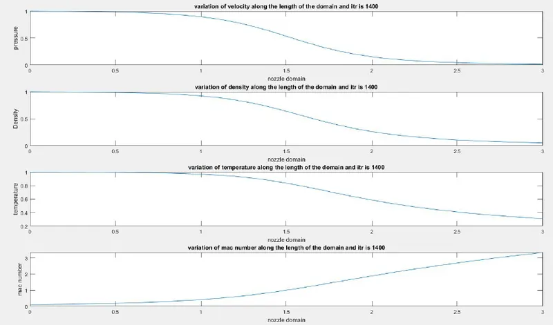
The above plot provides information regarding the variation of flow variables along the length of the domain. Pressure, Density and Temperature decrease along the length of the domain, whereas the Mac number increases along the length of the domain.

1.2 Mass flow rate in the nozzle at different time steps:

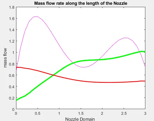
The above graph shows the mass flow rate at different time steps in the nozzle. After 600-700 time steps, the mass flow rate is constant for any time step above 700-time steps throughout the nozzle.

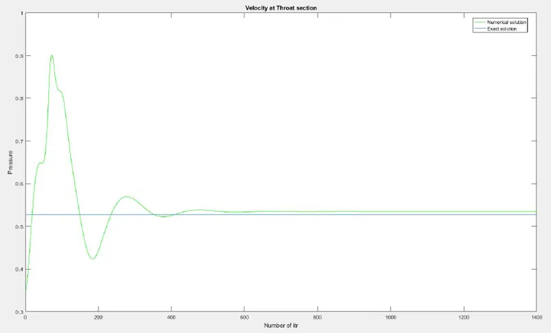
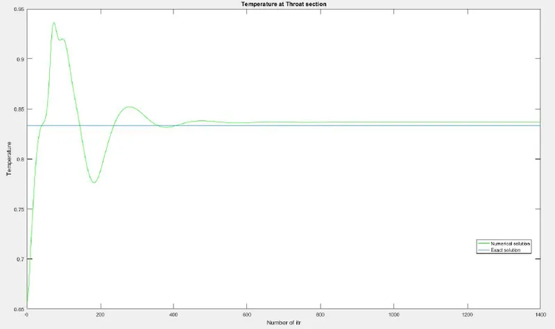
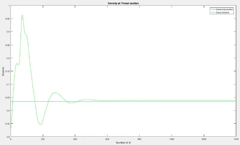
1.3 flow variables at the cross-section of the throat

Temperature:

Density:

Mac number:

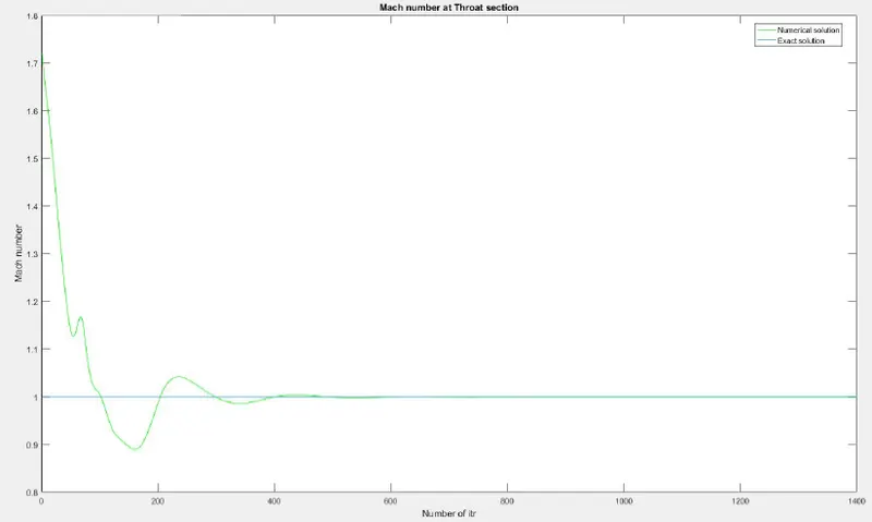
The above shows the variation of flow variables in the cross-section of the throat for different iterations. It has been observed after 400 it solution is getting stabilized, but there is a small difference between the exact and numerical solution.

2.Results for Non-conservative form:
Execution time:
184 sec
2.1 Variation of field variables along the length of the nozzle:

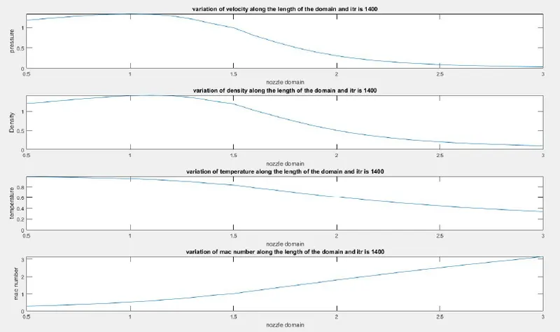
The above plot provides information regarding the variation of flow variables along the length of the domain. Pressure, Density and Temperature decrease along the length of the domain, whereas the Mac number increases along the length of the domain. For both forms of equations, the behaviour is the same.

1.2 Mass flow rate in the nozzle at different time steps:

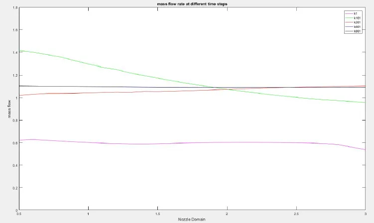
The above graph shows the mass flow rate at different time steps in the nozzle. After 600-700 time steps, the mass flow rate
is constant for any time step above 700-time steps throughout the nozzle.
when compared to the non-conserve method fluctuations are less.

2.3 flow variables at the cross-section of the throat:

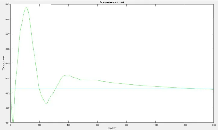
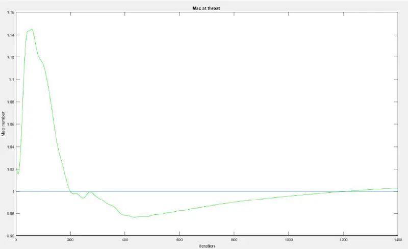
From the above graphs after 400-time steps solution starts getting constant whereas the variation from the exact solution
remains.

Temperature:

Mac:

Grid dependency test:

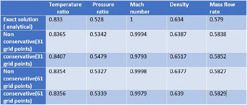
In order to conduct a grid dependency test, here two situations are considered one with 31 grid points and the other with 61 grid points. Values here shown are from the grid where the throat area lies. From the below table it can be seen that the increase in grid point will increase the accuracy but the run of the simulation also drastically increases with the increase in the number of grid points. It means that faster results in less are accurate.

Conclusion:

1. After comparing both the methods it has been seen that there are a lot more fluctuations in non-conservative flow when
compared to the conservative one.

2. After comparing both the forms in terms of execution time the non-conservative form is faster when compared to a
conservative form. The main reason is the conservative part has more mathematical calculations.

3. Non-Conservative form converges more quickly after 300 itr solution starts converging whereas conservative part requires 400 itr.

4. Complexity in solving the conservative form is more when compared to non-conservative since the conservative part has
more mathematical calculation when compared to other forms.