Week 5.1 - Mid term project - Solving the steady and unsteady 2D heat conduction problem

Let's solve the 2-D heat conduction equation for the steady and unsteady state using iterative
techniques such as Jacobi, gauss seidel, and successive over-relaxation method.

Concept:

This heat equation is needed to be solved by both explicit(where RHS terms are the terms of previous time steps) and
explicit(where RHS terms are if the next time steps)
Techniques used:

• For STEADY STATE(explicit method)
  • Jacobi method
  • Gauss Seidal method
  • SOR method
• For Transient using implicit method(iterative techniques)
  • Jacobi method
  • Gauss seidel
  • SOR method
• For Transient using Explicit method

For Steady State

we know that,

`frac{∂ T}{∂ t} = 0`

so the equation becomes,

(∂^2T)/(∂x^2)+(∂^2T)/(∂y^2) = 0

Discretizing the above equation

(del^2T)/(delx^2) = (T_(i-1,j)-2T_(i,j)+T_(i+1,j))/(Deltax^2)

(del^2T)/(dely^2) = (T_(i,j-1)-2T_(i,j)+T_(i,j+1))/(Deltay^2)

So the equation becomes

(T_(i-1,j)-2T_(i,j)+T_(i+1,j))/(Deltax^2) + (T_(i,j-1)-2T_(i,j)+T_(i,j+1))/(Deltay^2) = 0

As Nx=Ny , we consider

Deltax = Deltay

on rearranging the terms we get

`T_(i,j) = 1/4(T_(i-1,j)+T_(i+1,j)+T_(i,j-1)+T_(i,j+1))`

Let's code the main program

% steady state analysis
clear all
close all
clc
%inputs
nx=10; % number of grid points along x axis
ny=nx ;
x=linspace(0,1,nx);
dx=x(2)-x(1);
y=linspace(0,1,ny);
z=fliplr(y);
f=1.5;
iter=1;
t=ones([nx,ny])*298;
% Applying BC
t(1,1:nx)=600;
t(ny,1:nx)=900;
t(2:ny-1,1)=400;
t(2:ny-1,nx)=800;
% Creating a copy
told=t;
r1=t;
error=19;
tol=1e-4;
for iterative_solver=1:3
 while(error>tol)
 for i=2:nx-1
 for j=2:ny-1
 if(iterative_solver==1)
 t(i,j)=jacobi(t,told,i,j);
 elseif(iterative_solver==2)
 t(i,j)=GS(t,told,i,j);
 else
 t(i,j)=sor(t,told,i,j,f);
 end
 end
 end
 error=max(max(t-told));
 told=t;
 [u1,v1]=meshgrid(x,z);
 %plot

 if(iterative_solver==1)
 figure (1);
 contourf(u1,v1,t);
 [C,h]=contourf(u1,v1,t);
 colorbar;
 colormap(jet);
 clabel(C,h);
 xlabel('x-axis');
 ylabel('y-axis');
 title_text=sprintf('jacobi iterantion number=%d',iter);
 title(title_text);
 pause(0.003);
 elseif(iterative_solver==2)

 figure (2);
 contourf(u1,v1,t);
[C,h]=contourf(u1,v1,t);

[C,h] contourf(u1,v1;t);
 colorbar;
 colormap(jet);
 clabel(C,h);
 xlabel('x-axis');
 ylabel('y-axis');
 title_text=sprintf('GS iterantion number=%d',iter);
 title(title_text);
 pause(0.003);
 else
 figure (3);
 [C,h]=contourf(u1,v1,t);
 colorbar;
 colormap(jet);
 clabel(C,h);
 xlabel('x-axis');
 ylabel('y-axis');
 title_text=sprintf('sor iterantion number=%d',iter);
 title(title_text);
 pause(0.003);
 end
 iter=iter+1;
 end
error=19;
iter=1;
t=r1;
told=r1;
 end

function code for jacobi:

function out = jacobi(t,told,i,j)
 out=0.25*((told(i,j-1)+told(i,j+1)+told(i-1,j)+told(i+1,j)));
end

function code for GS:

function out = GS(t,told,i,j)
 out

function code for SOR:

Results:

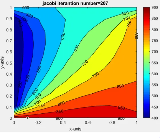
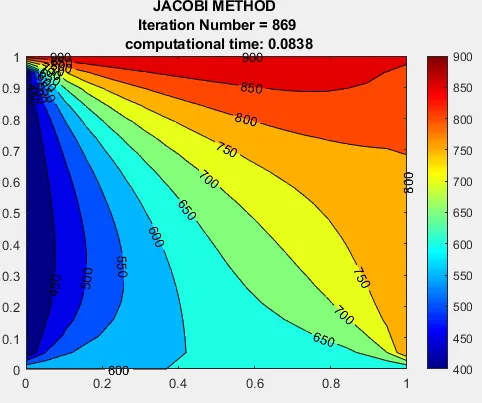
jacobi method:

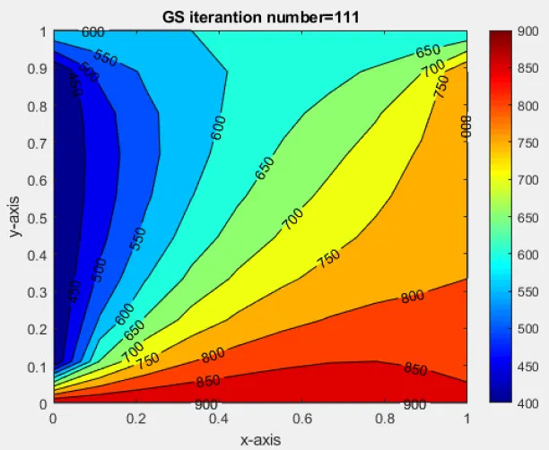
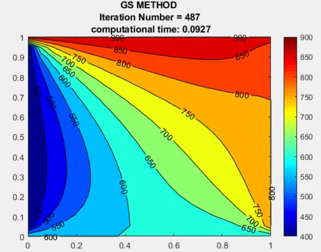
GS method:

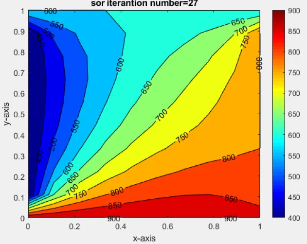
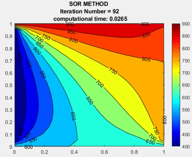
SOR method:

Conclusion :

From the above results we can conclude that the SOR is the fastest method as it solves the equations in just 27 iterations, this
number of iteration and the stability of the solution depends on the relaxation factor (in sor) value of relaxation factor less than
0 is called the under-relaxation which will increase the number of iteration even greater than Jacobi
and too much over relaxation will blow up the solution it is essential to choose the value of relaxation factor carefully

Let's use the Transient Method

2-D heat equation for an unsteady state is given by,

`alpha((del^2T)/(delx^2)+(del^2T)/(dely^2)) = (delT)/(delt)`

Discretizing the spacial terms
we get,

`(del^2T)/(delx^2) = (T_(i-1,j)-2T_(i,j)+T_(i+1,j))/(Deltax^2)`

`(del^2T)/(dely^2) = (T_(i,j-1)-2T_(i,j)+T_(i,j+1))/(Deltay^2)`

Discretizing the time derivative,

`(delT)/(delt) = ((T^(n+1))_(i,j)-(T^(n))_(i,j))/(Deltat)`

so now equation becomes,
for explicit method

`alpha((T_(i-1,j)-2T_(i,j)+T_(i+1,j))^(n)/(Deltax^2) + (T_(i,j-1)-2T_(i,j)+T_(i,j+1))^(n)/(Deltay^2)) = ((T^(n+1))_(i,j)-(T^(n))_(i,j))/(Deltat)`

after rearranging the above equation becomes,

`(T^(n+1))_(i,j) = lambda((T^n)_(i-1,j) + (T^n)_(i,j-1) ) + [1 -4lambda](T^n)_(i,j) + lambda( (T^n)_(i+1,j) + (T^n)_(i,j+1))`

Where,

`lambda = (alpha*Deltat)/(Deltax^2)`

lamda is also called as the CFL number, CFL number is used to check the stability of the solution.
alpha is the convective coefficient

Let's code for explicit method

% Transient state problem(explicit)
clear all
close all
clc
%basic inputs
nx=10;
ny=nx;
x=linspace(0,1,nx);
dx=x(2)-x(1);
y=linspace(0,1,ny);
dy=y(2)-y(1);
%convective coefficient
c=1e-4;
%NUMBRER OF TIME STPES
 nt=200;
%TIME STEP
dt=32;
%CFL NUMBER
k= (c*dt)/dx^2;
t=ones([nx,ny])*673;
%applying the boundary conditions
t(1,1:nx)=600;
t(ny,1:nx)=900;
t(2:ny-1,1)=400;
t(2:ny-1,nx)=800;
told=t;
[xx,yy]=meshgrid(x,y);
tic
iter=1;
 for p=1:nt
 for i=2:nx-1
 for j=2:ny-1
 t(i,j)= k*(told(i-1,j) + told(i,j-1) + told(i+1,j) + told(i,j+1)) + (1-4*k)*told(i,j);
 end
 end

 error=max(abs(told-t));
 told=t;
 iter=iter+1;
 end
time=toc;
figure (1);
[C,h]=contourf(xx,yy,t);
colorbar;
colormap(jet);
clabel(C,h);
title(sprintf('2D Unsteady state heat conduction (Explicit Method) \n Computation Time: %0.4f \n CFL Number: 
%0.4f \n iterations=%d',time,k,iter));
xlabel('xx');
ylabel('yy');

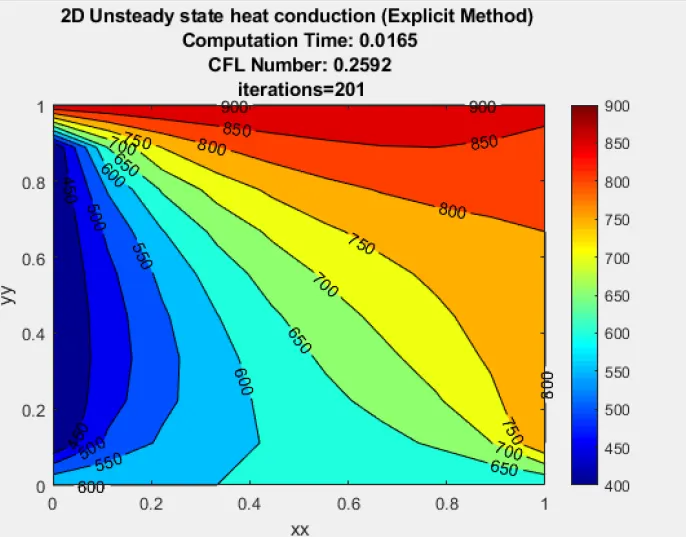
Results:

For implicit method
we know that

`T_p^(n+1) = (T_p^n + k1(T_L^(n+1)+T_R^(n+1))+k2(T_T^(n+1)+T_B^(n+1)))/(1+2k1+2k2)`

Let's code for implicit method

GS:

SOR:

Observation and result:

• as we can see from the results of the EXPLICIT and IMPLICIT method, the explicit method is much faster than the implicit method ( in comparison to all three iterative techniques)
• the computational time for the explicit method is 0.0165 with 201 iteration
• the fastest method is implicit is the sor with the computational time of 0.0265 with 92 iteration
• but from the explicit and implicit method, implicit is much accurate as it uses various iterative solvers to converge the solution and above this, it uses all values from the entire domain.
• another great technique to improve the accuracy of the implicit method is to use the inverse matrix technique