Week 3 - Taylor table method and Matlab code

1. Fourth-order approximation of second-order derivative by using ''Central Differencing scheme''

Number of Grid Points = Order of Error + Order of Derivative-1

Therefore,= 4+2-1 = 5

The second-order accurate approximation is :

∂u/∂x = a*f(i-2)+b*f(i-1)+c*f(i)+d*f(i+1)+e*f(i+2)

Taylor's table shown below:

	f(i)	Δx*f'(i)	Δx^2*f''(i)	Δx^3*f'''(i)	Δx^4*f''''(i)
af(i-2)	a	-2a	4a/2	-8a/6	16a/24
bf(i-1)	b	-b	b/2	-b/6	b/24
cf(i)	c	0	0	0	0
df(i+1)	d	d	d/2	d/6	d/24
ef(i+2)	e	2e	4e/2	8e/6	16e/24
Sum	0	0	1	0	0

Taylor’s table the sum of 1,2,4,5 column is taken to be zero and the sum of 3rd the column is equated to 1 for Central Differencing scheme.

Taylor series expansion is,

f(i-2) = f(i) +[f’(i)*(-2Δx)/1!] + [f’’(i)*(-2*Δx)/2!] + [f’’’(i)*(-2*Δx)/3!] + [f(i)*(-2*Δx)/4!]+...

f(i-1) = f(i) +[f’(i)*(-1Δx)/1!] + [f’’(i)*(-1*Δx)/2!] + [f’’’(i)*(-1*Δx)/3!] + [f(i)*(-1*Δx)/4!]+...

f(i) = f(i)

f(i+1) = f(i) +[f’(i)*(1Δx)/1!] + [f’’(i)*(1*Δx)/2!] + [f’’’(i)*(1*Δx)/3!] + [f(i)*(1*Δx)/4!]+...

f(i+2) = f(i) +[f’(i)*(2Δx)/1!] + [f’’(i)*(2*Δx)/2!] + [f’’’(i)*(2*Δx)/3!] + [f(i)*(2*Δx)/4!]+...

Getting equations from Taylor’s Table,

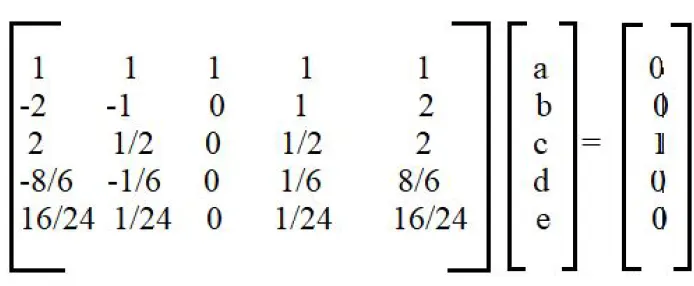
a + b + c + d + e = 0
-2a – b + 0 + d + 2e = 0
2a + b/2 + 0 + d/2 + 2e = 1
-8a/6 - b/6 + 0 + d/6 + 8e/6 = 0
16a/24 + b/24 + 0 +d/24 + 16e/24 = 0

In Matrix format

Therefor,

a = -0.0833 b = 1.3333 c = -2.5000 d = 1.3333 e = -0.0833

Skewed Right sided difference Scheme :

The second-order accurate approximation is

∂u/∂x = a*f(i)+b*f(i+1)+c*f(i+2)+d*f(i+3)+e*f(i+4)+f*f(i+5)

Taylor's table shown below:

	f(i)	Δx*f'(i)	Δx^2*f''(i)	Δx^3*f'''(i)	Δx^4*f''''(i)	Δx^5*f'''''(i)
a*f(i)	a	0	0	0	0	0
b*f(i+1)	b	b	b/2	b/6	b/24	b/120
c*f(i+2)	c	2c	4c/2	8c/6	16c/24	32c/120
d*f(i+3)	d	3d	9d/2	27d/6	81d/24	243d/120
e*f(i+4)	e	4e	16e/2	64e/6	256e/24	1024e/120
f*f(i+5)	f	5f	25f/2	125f/6	625f/24	3125e/120
Sum	0	0	1	0	0

the sum of 1st,2nd,4th,5th,6th column is taken to be zero and the sum of 3 columns is equated to 1

Taylor series expansion is :

f(i) = f(i)
f(i+1) = f(i) +[f’(i)*(1Δx)/1!] + [f’’(i)*(1*Δx)/2!] + [f’’’(i)*(1*Δx)/3!] + [f(i)*(1*Δx)/4!] +..............................
f(i+2) = f(i) +[f’(i)*(2Δx)/1!] + [f’’(i)*(2*Δx)/2!] + [f’’’(i)*(2*Δx)/3!] + [f(i)*(2*Δx)/4!] +..............................
f(i+3) = f(i) +[f’(i)*(3Δx)/1!] + [f’’(i)*(3*Δx)/2!] + [f’’’(i)*(3*Δx)/3!] + [f(i)*(3*Δx)/4!] +..............................
f(i+4) = f(i) +[f’(i)*(4Δx)/1!] + [f’’(i)*(4*Δx)/2!] + [f’’’(i)*(4*Δx)/3!] + [f(i)*(4*Δx)/4!] +..............................
f(i+5) = f(i) +[f’(i)*(5Δx)/1!] + [f’’(i)*(5*Δx)/2!] + [f’’’(i)*(5*Δx)/3!] + [f(i)*(5*Δx)/4!] +..............................

Getting equations from Taylor’s Table :

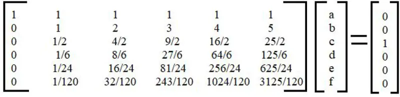
a + b + c + d + e + f = 0
0 + b + 2c + 3d + 4e + 5f = 0
0 + b/2 + 4c/2 + 9d/2 + 16e/2 + 25f/2 = 1
0 + b/6 + 8c/6 + 27d/6 + 64e/6 + 125f/6 = 0
0 + b/24 + 16c/24 + 81d/24 + 256e/24 + 625f/24 = 0
0 + b/120+ 32c/120 +243d/120 + 1024e/120+ 3125f/120 = 0

In Matrix format

Solving the above Matrix

a = 3.75000

b = -12.83333

c = 17.83333

d =-13.0000

e = 5.08333

f = -0.83333

Skewed Left-sided difference Scheme :

The second-order accurate approximation is,

∂u/∂x = a*f(i-5)+b*f(i-4)+c*f(i-3)+d*f(i-2)+e*f(i-1)+f*f(i)

Taylor's table shown below :

	f(i)	Δx*f'(i)	Δx^2*f''(i)	Δx^3*f'''(i)	Δx^4*f''''(i)	Δx^5*f'''''(i)
a*f(i-5)	a	-5a	25a/2	-125a/6	625a/24	-3125a/120
b*f(i-4)	b	-4b	16b/2	-64b/6	256b/24	-1024b/120
c*f(i-3)	c	-3c	9c/2	-27c/6	81c/24	-243c/120
d*f(i-2)	d	-2d	4d/2	-8d/6	16d/24	-32d/120
e*f(i-1)	e	-e	e/2	-e/6	e/24	-e/120
f*f(i)	f	0	0	0	0	0
Sum	0	0	1	0	0	0

sum of 1 ,2 , 4 ,5 ,6 column is taken to be zero and the sum of 3 column is equated to 1.

Taylor series expansion is written as,

f(i-5) = f(i) +[f’(i)*(-5Δx)/1!] + [f’’(i)*(-5*Δx) /2!] + [f’’’(i)*(-5*Δx) /3!] + [f (i)*(-5*Δx) /4!] + ...
f(i-4) = f(i) +[f’(i)*(-4Δx)/1!] + [f’’(i)*(-4*Δx) /2!] + [f’’’(i)*(-4*Δx) /3!] + [f (i)*(-4*Δx) /4!] + ...
f(i-3) = f(i) +[f’(i)*(-3Δx)/1!] + [f’’(i)*(-3*Δx) /2!] + [f’’’(i)*(-3*Δx) /3!] + [f (i)*(-3*Δx) /4!] + ...
f(i-2) = f(i) +[f’(i)*(-2Δx)/1!] + [f’’(i)*(-2*Δx) /2!] + [f’’’(i)*(-2*Δx) /3!] + [f (i)*(-2*Δx) /4!] + ...
f(i-1) = f(i) +[f’(i)*(-1Δx)/1!] + [f’’(i)*(-1*Δx) /2!] + [f’’’(i)*(-1*Δx) /3!] + [f (i)*(-1*Δx) /4!] + ...
f(i) = f(i)

Getting equations from Taylor’s Table

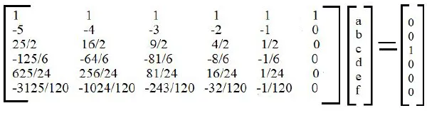
a + b + c + d + e + f = 0

-5a - 4b - 3c - 2d – e + 0f=0

25a/2 + 16b/2 + 9c/2 + 4d/2 + e/2 + 0f = 1

-125a/6 – 64b/6 – 81c/6 – 8d/6 – e/6 + 0f = 0

625a/24 + 256b/24 +81c/24 + 16d/24 + e/24 + 0f = 0

-3125a/120 - 1024b/120 - 243c/120 - 32d/120 – e/120 +0f = 0

In Matrix format

Solving this Metrix,

a = 0.091046 b = -0.330888 c = -0.058691 d = 2.250941 e = -3.457487 f = 1.505079

Matlab Code:

1) Error find out the program

function [error] = Week_3_taylor_table_fun(x,dx) 

%program to evaluate exp(x)*cos(x) 

%First Finding analytical derivative for the given equation 
%f(x) = (e^x)*cos(x) 
%f'(x) = (e^x)*cos(x) - (e^x)*sin(x) 
%f''(x) = -2*(e^x)*sin(x) 

% x = 0.5; dx = 0.1;

analytical_derivative = (-2).*(exp(x)).*(sin(x)); 

%solving using numerical discretization of fourth order 
%central differencing = f''(x) = (-f(i+2) + 16f(i+1) - 30f(i) + 16f(i-1) - f(i-2))/(12*dx^2) 

central_D = (-((exp(x+2*dx))*cos(x+2*dx)) + 16*((exp(x+dx))*cos(x+dx)) - 30* ((exp(x))*cos(x)) + 16*((exp(x-dx))*cos(x-dx)) - ((exp(x-2*dx))*cos(x-2*dx)))/(12*dx^2); 

right_skewed = (45*((exp(x))*cos(x)) - 154*((exp(x+dx))*cos(x+dx)) + 214* ((exp(x+2*dx))*cos(x+2*dx)) - 156*((exp(x+3*dx))*cos(x+3*dx)) + 61* ((exp(x+4*dx))*cos(x+4*dx)) -10*((exp(x+5*dx))*cos(x+5*dx)))/(12*dx^2); 

left_skewed = (45*((exp(x))*cos(x)) - 154*((exp(x-dx))*cos(x-dx)) + 214* ((exp(x-2*dx))*cos(x-2*dx)) - 156*((exp(x-3*dx))*cos(x-3*dx)) + 61* ((exp(x-4*dx))*cos(x-4*dx)) -10*((exp(x-5*dx))*cos(x-5*dx)))/(12*dx^2); 

error(1) = abs(central_D - analytical_derivative);

error(2) = abs(right_skewed - analytical_derivative); 

error(3) = abs(left_skewed - analytical_derivative); 

end

2) Program for ploat

clc 

%code to compare absolute error between three schemes and analytical error 
x = pi/4; 
dx = linspace(pi/4,pi/300,70);

%preallocating for speed 
central_difference_error = zeros(1,length(dx)); 
right_skewed_error = zeros(1,length(dx)); 
left_skewed_error = zeros(1,length(dx)); 

for i = 1:length(dx)
    
    error = Week_3_taylor_table_fun(x,dx(i)); 
    central_difference_error(i) = error(1); 
    right_skewed_error(i) = error(2); 
    left_skewed_error(i) = error(3); 
end

figure(1) 
loglog(dx,central_difference_error,'-db') 
hold on 
loglog(dx,right_skewed_error,'-sblack') 
hold on 
loglog(dx,left_skewed_error,'-or') 
xlabel('dx') 
ylabel('Absolute Error') 
legend('Central Difference of 4th Order','Skewed Right Sided Difference of 4th Order','Skewed Left Sided Difference of 4th Order') 
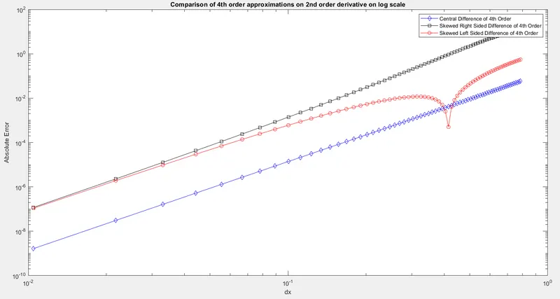
title('Comparison of 4th order approximations on 2nd order derivative on log scale') 

figure(2) 
plot(dx,central_difference_error,'-db') 
hold on 
plot(dx,right_skewed_error,'-sblack') 
hold on 
plot(dx,left_skewed_error,'-or') 
xlabel('dx') 
ylabel('Absolute Error') 
legend('Central Difference of 4th Order','Skewed Right Sided Difference of 4th Order','Skewed Left Sided Difference of 4th Order') 

%Derivation and approximation of fourth order approximation schemes ( Central difference, Right-skewed, Left-skewed) for second order derivative and their error comparison for function e^(x)*cos(x) : S…
title('Comparison of 4th order approximations on 2nd order derivative on normal scale')

Result Plot :

1) Comparison of 4th order on 2nd order derivative.

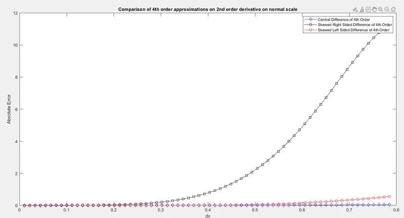
2) same comparison on a log scale