Week 7 - Auto ignition using Cantera

PART I

Use the same reactor network code as shown in the video to simulate the Auto Ignition Time for Methane under the following conditions, (simulation time = 10 secs)

• Plot the variation of Auto Ignition time of Methane with a constant temperature of 1250K and pressure varying from 1 to 5 atm.
• Plot the variation of Auto Ignition time of Methane with a constant pressure of 5 atm and temperature varying from 950K to 1450K.

NOTE:

Auto Ignition time is the time when the temperature of the reactor is Initial Temperature plus 400K.

Auto Ignition time: It's the time taken for the combustion to happen form the injection of the methane into the combustor. The combustion happens all of by without any external agencies being involved. After the autoignition delay time the temperature in the reactor or combustor will be higest.

Plot the variation of Auto Ignition time of Methane with a constant temperature of 1250K and pressure varying from 1 to 5 atm.

Here the variatio of the Auto ignition time of methane has to be understood with variation of the inlet pressure at a fixed temperature of 1250K.

Programming Procedure:

• Declare the soulution object of the cantera class by name gas
• Declaring the initial and final pressure for the simulation with the temperature of 1250K
• Declare an Reactor of the gas object
• Declare an variable name states of the class solutionArray
• Writing an nested for loop to cover over all the pressure and all the values of the time with deltat =1e-03
• Advancce the simuation for every 1e-03 time step and append the solution to the solution state array, which is the of the class solution Array
• store the temperature array of the solutionArray class to a new matrix.
• Once the solution is run over all the pressure and all the time, a new function is developed which perfirms the array maniplation to determine the auto ignition time and termperature.
• This particular function is written in such a generic format that it can handle all the three problems asked in the challenge.
• At the end all the function files are

def Auto_Ignition_Delaytime_Consttemp(Temperature, time, temp_old, case):
	dummy1=[]
	dummy2=[]

	[r,c]=Temperature.shape

	if (case ==1):	
		dummy3=1250	
		for col in range (5):
			t_old=dummy3	
			for row in range (len(Temperature)):
				t_new=Temperature[row, col]
				#b1=Temperature[row+1, col]
				tau=time[row, col]+0.001 # This because the storing of time happens on the first iteration
				if ((t_new-t_old) >= 400):				
					dummy1.append(t_new)
					dummy2.append (tau)
				t_old=t_new
	if (case ==2):
		dummy3=np.linspace(950, 1450, 10)

		for col in range (10):
			t_old=dummy3[col]	
			for row in range (len(Temperature)):
				t_new=Temperature[row, col]
				#b1=Temperature[row+1, col]
				tau=time[row, col]+0.001 # This because the storing of time happens on the first iteration
				if ((t_new-t_old) >= 400):				
					dummy1.append(t_new) # Temperaute
					dummy2.append (tau)  # Time in [sec]
				t_old=t_new

	return dummy1, dummy2

The above the function file used for all the cases.

def Case_I ():

	gas =cnt.Solution('gri30.yaml')
	P_ini=cnt.one_atm
	P_final=5*cnt.one_atm
	#time_ini=0    # Seconds
	#time_final=10 # Seconds
	#Integration_time_step=1e-03
	#no_time_steps=int((time_final-time_ini)/(Integration_time_step))
	Pressure=np.linspace(P_ini, P_final, 5)
	time_simulation=np.zeros((10000, len(Pressure)), dtype=float)
	temp_New=np.zeros((10000, len(Pressure)))

	itr=0
	for i in Pressure:
		Temperature=1250 # Temperature
		gas.TPX=Temperature, i, {'CH4':1, 'N2':7.52, 'O2': 2}
		Reactor=cnt.IdealGasReactor(gas)
		Simulation=cnt.ReactorNet([Reactor])
		states=cnt.SolutionArray(gas, extra=['time_in_ms', 't'])
		time=0.0000
		T_old=Temperature

		for j in range(10000):
			time+=1e-03
			time_simulation[j,itr]=time
			Simulation.advance(time)
			states.append(Reactor.thermo.state, time_in_ms=time*1e-03, t=time)
			# Logic observed in online
   
		temp_New[:,itr]=states.T

		itr=itr+1
	[a1, a2]=Auto_Ignition_Delaytime_Consttemp(temp_New, time_simulation,Temperature, 1 )
	return a1, a2, time_simulation, Pressure, temp_New

Lines to call the function files for case_01

[a1, a2, time_simulation_1, Pressure, temp_New]=Case_I()

plt.figure(1)
plt.plot(time_simulation_1[:,1], temp_New)
plt.xlabel('time of simulation [ms]')
plt.ylabel('The Temperature [K]')
plt.legend(['1 atm','2 atm', '3 atm', '4 atm', '5 atm']) 
plt.grid ()
plt.show()

plt.figure(2)
plt.plot(Pressure, a2, 'o-r')
plt.xlabel('Pressure [pa]')
plt.ylabel('The ignition time delay [sec]')
plt.grid ()
plt.show()

The output obtained are:

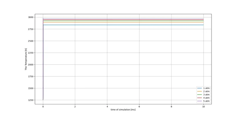
Variation of the temperature with time is shown in the figure above: It can be seen that initially the temperature is initialy 1250K and reaches the temperature in the range of 2759 to 3000K for the pressure rangeing from 1atm to 5 atm. The higher temeprature is obtained at the higher pressures and that is depicted in the plot above.

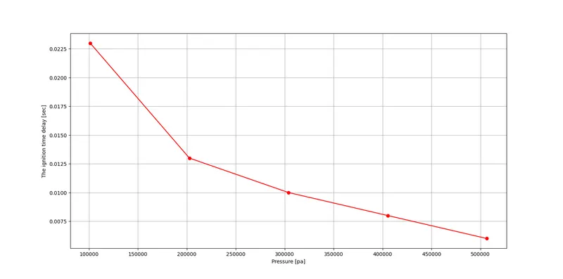
It can be seen that the ignition time i.e time required for combustion to sustain decreases with the increase in the pressure. Pressure is higher Temperature will be higher for the gas mixture and the time taken for the combustion to start will be lower.

• Plot the variation of Auto Ignition time of Methane with a constant pressure of 5 atm and temperature varying from 950K to 1450K.

############################### Defining the function file for case 2########################################################
def Case_II ():

	gas =cnt.Solution('gri30.yaml')
	pressure=5*cnt.one_atm
	
	#time_ini=0    # Seconds
	#time_final=10 # Seconds
	
	#Integration_time_step=1e-03

	#no_time_steps=int((time_final-time_ini)/(Integration_time_step))
	
	T_ini=950
	
	T_final=1450

	Temperature=np.linspace(T_ini, T_final, 10)
	Tempe=np.linspace(T_ini, T_final, 10)

 
	time_simulation=np.zeros((10000, len(Temperature)), dtype=float)
	
	temp_New=np.zeros((10000, len(Temperature)))

	itr=0

	for i in Temperature:
		Temperature=i # Temperature
		gas.TPX=Temperature, pressure, {'CH4':1, 'N2':7.52, 'O2': 2}
		Reactor=cnt.IdealGasReactor(gas)
		Simulation=cnt.ReactorNet([Reactor])
		states=cnt.SolutionArray(gas, extra=['time_in_ms', 't'])
		time=0.0000
		T_old=Temperature

		for j in range(10000):
			time+=1e-03
			time_simulation[j,itr]=time
			Simulation.advance(time)
			states.append(Reactor.thermo.state, time_in_ms=time*1e-03, t=time)
			# Logic observed in online
		
		temp_New[:,itr]=states.T
		
		itr=itr+1
		#temp_New=states.T

	[a1, a2]=Auto_Ignition_Delaytime_Consttemp(temp_New, time_simulation,Temperature, 2)

	return a1, a2, time_simulation, Tempe, temp_New

########################################### CALLING THE CASE II TO PLOT THE MOLAR CONCENTRATIONS ################################################


[a1, a2, time_simulation_1, Tempe, temp_New]=Case_II()

 ##3 making the plots for case 2

plt.figure(3)
plt.plot(time_simulation_1[:,1], temp_New)
plt.xlabel('time of simulation [ms]')
plt.ylabel('The Temperature [K]')
#plt.legend(['1 atm','2 atm', '3 atm', '4 atm', '5 atm']) 
plt.grid ()
plt.show()


print(Tempe)
plt.figure(4)
plt.plot(Tempe, a2, 'o-r')
plt.xlabel('Temperature [K]')
plt.ylabel('The ignition time delay [sec]')
plt.grid ()
plt.show()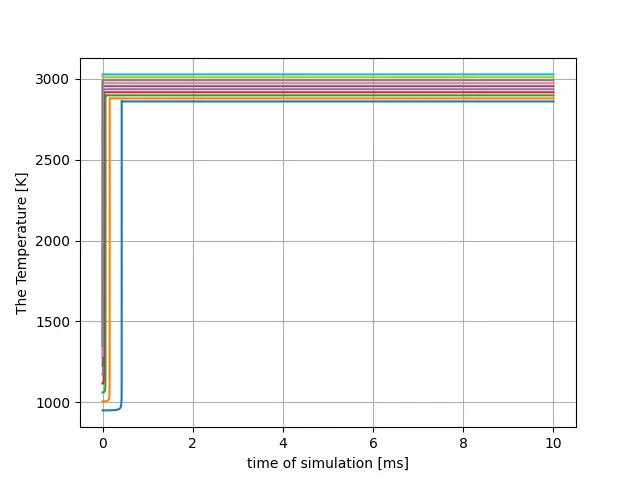

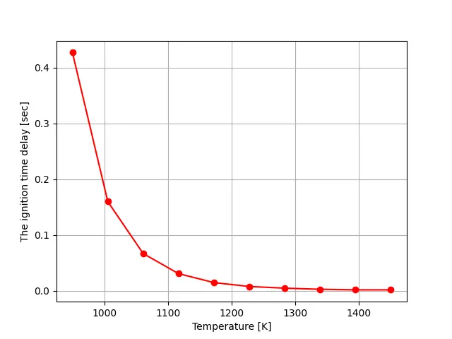
From the above two figures it can be seen that at specific pressure with increase in teh temperature the ignition delay time will be lower at the higher temepratures i.e. both are inversely realted.

PART II

Further, observe and print the rate of change of molar concentrations of the given elements "H2O, O2, OH" with respect to the time, (simulation time = 10 secs)

Explain the behavior of the graph for 2 cases,

• When Temperature is 1000K and pressure 5 bar
• When Temperature is 500K and pressure 5 bar

here we are not interested in the variation of termperature, we are interested to visualize the variation of the concentrations of the elements which are fomed during ther reaction:

def case_III ():
	gas =cnt.Solution('gri30.yaml')
	pressure=5*cnt.one_atm
	
	time_ini=0    # Seconds
	time_final=10 # Seconds
	
	Integration_time_step=1e-03

	no_time_steps=int((time_final-time_ini)/(Integration_time_step))
	
	Temperature=[500, 1000]

	Tempe=Temperature

	delay_time=[]

	time_simulation=np.zeros((no_time_steps, len(Temperature)), dtype=float)
	
	temp_New=np.zeros((no_time_steps, len(Temperature)))

	Mole_data_h2o=np.zeros((no_time_steps, 2))
	Mole_data_o2=np.zeros((no_time_steps, 2))
	Mole_data_oh=np.zeros((no_time_steps, 2))

	itr=0

	for i in Temperature:
		Temperature=i # Temperature
		gas.TPX=Temperature, pressure, {'CH4':1, 'N2':7.52, 'O2': 2}
		Reactor=cnt.IdealGasReactor(gas)
		Simulation=cnt.ReactorNet([Reactor])
		states=cnt.SolutionArray(gas, extra=['time_in_ms', 't'])
		time=0.0000
		T_old=Temperature

		for j in range(no_time_steps):
			time+=1e-03
			time_simulation[j,itr]=time
			Simulation.advance(time)
			states.append(Reactor.thermo.state, time_in_ms=time*1e-03, t=time)
			
		
		temp_New[:,itr]=states.T
		Mole_data_h2o[:, itr]=states.X[:, gas.species_index('H2O')]
		Mole_data_o2 [:, itr]=states.X[:, gas.species_index('O2')]
		Mole_data_oh [:, itr]=states.X[:, gas.species_index('OH')]

		itr=itr+1
		#temp_New=states.T
	   
	#[a1, a2]=Auto_Ignition_Delaytime_Consttemp(temp_New, time_simulation,Temperature, 2)

	return time_simulation, Tempe, temp_New, Mole_data_h2o, Mole_data_o2, Mole_data_oh

########################################### CALLING THE CASE III TO PLOT THE MOLAR CONCENTRATIONS ################################################

[time_simulation, Tempe, temp_New, Mole_data_h2o, Mole_data_o2, Mole_data_oh]=case_III()

plt.figure(5)
plt.suptitle("variation of mole fraction of H20, OH and O2 at 500K for first 10 sec")

plt.subplot(2,2,1)

plt.plot(time_simulation[:,0], temp_New[:,0], 'r-')
plt.grid ()
plt.legend(['Temperature=500k'])
plt.xlabel('Time [sec]')
plt.ylabel('Temperature')

plt.subplot(2,2,2)
plt.plot(time_simulation[:,0], Mole_data_h2o[:,0], color='darkblue', linestyle='-', linewidth=2)
plt.grid ()
plt.legend(['Temperature=500k'])
plt.xlabel('Time [sec]')
plt.ylabel('H20 Mole fraction')
plt.subplot(2,2,3)
plt.plot(time_simulation[:,0], Mole_data_o2[:,0],color='m', linestyle='-',linewidth=2)
plt.grid ()
plt.legend(['Temperature=500k'])
plt.xlabel('Time [sec]')
plt.ylabel('O2 Mole fraction')
plt.subplot(2,2,4)
plt.plot(time_simulation[:,0], Mole_data_oh[:,0],color='g', linestyle='-',linewidth=2)
plt.grid ()
plt.legend(['Temperature=500k'])
plt.xlabel('Time [sec]')
plt.ylabel('OH Mole fraction')

plt.show()


plt.figure(6)
plt.suptitle("variation of mole fraction of H20, OH and O2 at 100K for first 10 sec")

plt.subplot(2,2,1)

plt.plot(time_simulation[:,0], temp_New[:,1], 'r-')
plt.grid ()
plt.legend(['Temperature=1000k'])
plt.xlabel('Time [sec]')
plt.ylabel('Temperature')

plt.subplot(2,2,2)
plt.plot(time_simulation[:,0], Mole_data_h2o[:,1], color='darkblue', linestyle='-', linewidth=2)
plt.grid ()
plt.legend(['Temperature=1000k'])
plt.xlabel('Time [sec]')
plt.ylabel('H20 Mole fraction')
plt.subplot(2,2,3)
plt.plot(time_simulation[:,0], Mole_data_o2[:,1],color='m', linestyle='-',linewidth=2)
plt.grid ()
plt.legend(['Temperature=1000k'])
plt.xlabel('Time [sec]')
plt.ylabel('O2 Mole fraction')
plt.subplot(2,2,4)
plt.plot(time_simulation[:,0], Mole_data_oh[:,1],color='g', linestyle='-',linewidth=2)
plt.grid ()
plt.legend(['Temperature=1000k'])
plt.xlabel('Time [sec]')
plt.ylabel('OH Mole fraction')

plt.show()

here we will be observing the variation of the molefractions as a function of tme:

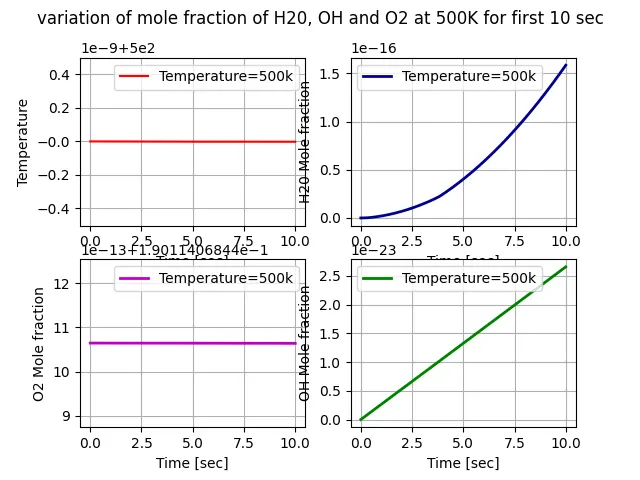
since the ititial temperature is too low, we can see that the H20 moles formation is very low. The OH formation and O2 decomposition is also way to low i.e. in the order of 1e-12 to 15.

Where as in the case of 1000K we have the following plot:

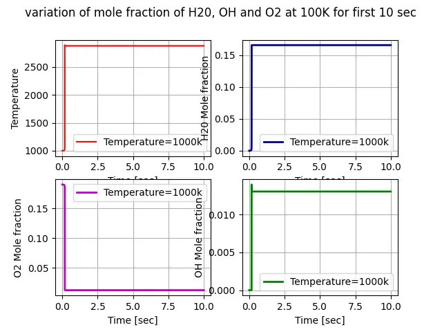
the temperaure is higher and the combustion intiates and the autoignition temperature is obtained. It can be seen that Oxygen moes are decreasing and the moles of the products i.e. OH and H20 are increaseing.