Week 7 - Auto ignition using Cantera

Aim --> Autoignition using Cantera

Autoignition is the lowest temperature at which the combustion takes place. It is the time at which the temperature of the mixture is 400 K above the initial temperature of the reactant mixture. The time duration before that is the ignition delay period. Ignition delay is a function of temperature(initial), pressure and species concentration. The study of Ignition delay is important in low-temperature combustion. This is because of the Negative-Temperature-coefficient (NTC) region.

PART I

Use the same reactor network code as shown in the video to simulate the Auto Ignition Time for Methane under the following conditions, (simulation time = 10 secs)

• Plot the variation of Auto Ignition time of Methane with a constant temperature of 1250K and pressure varying from 1 to 5 atm.

import numpy as nu
import matplotlib.pyplot as plt
import cantera as ct
import sys

T=1250
P=101325
def f(T,P):
   gas = ct.Solution('gri30.xml')
   gas.TPX = T, P, {'CH4':1,'O2':2,'N2':7.52}
   r=ct.IdealGasReactor(gas)
   sim=ct.ReactorNet([r])
   time=0.0
   Ignition_delay = []
   states=ct.SolutionArray(gas, extra=['time_in_ms','t'])
   for n in range(1000):
      time += 1e-3 # 1 ms [Cantera chooses its own time step]
      sim.advance(time)
      states.append(r.thermo.state, time_in_ms=time*1e-3, t=time)      
   for i in range(len(states.T)):
      if states.T[i] >= 1650:
         Ignition_delay.append(states.t[i])
         break             
   return states,Ignition_delay
states_1, I1=f(T,P)
states_2, I2=f(T,2*P)
states_3, I3=f(T,3*P)
states_4, I4=f(T,4*P)
states_5, I5=f(T,5*P)
Pressure = [1, 2, 3, 4, 5]
I=[I1, I2, I3, I4, I5]

plt.figure(1)
plt.plot(states_1.T)
plt.plot(states_2.T)
plt.plot(states_3.T)
plt.plot(states_4.T)
plt.plot(states_5.T)
plt.xlabel('Time in ms')
plt.ylabel('Temperature')
plt.title('Temperature variation wrt time')
plt.legend(['1 atm','2 atm','3 atm','4 atm','5 atm'])
plt.figure(2)
plt.plot(Pressure,I)
plt.title('Ignition delay variation wrt Pressure')
plt.xlabel('Pressure in bar')
plt.ylabel('Time in s')
plt.show()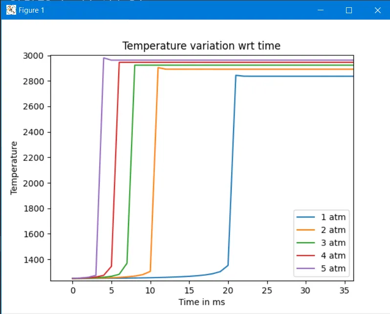

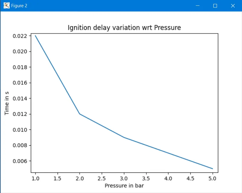
We can see as the pressure increases Ignition delay period decreases.

• Plot the variation of Auto Ignition time of Methane with a constant pressure of 5 atm and temperature varying from 950K to 1450K.

import numpy as nu
import matplotlib.pyplot as plt
import cantera as ct
import sys

T1=950
T2=1050
T3=1150
T4=1250
T5=1350
T6=1450
P=5*101325
def f(T,P):
   gas = ct.Solution('gri30.xml')
   gas.TPX = T, P, {'CH4':1,'O2':2,'N2':7.52}
   r=ct.IdealGasReactor(gas)
   sim=ct.ReactorNet([r])
   time=0.0
   Ignition_delay = []
   states=ct.SolutionArray(gas, extra=['time_in_ms','t'])
   for n in range(1000):
      time += 1e-3 # 1 ms [Cantera chooses its own time step]
      sim.advance(time)
      states.append(r.thermo.state, time_in_ms=time*1e-3, t=time)      
   for i in range(len(states.T)):
      if states.T[i] >= 1650:
         Ignition_delay.append(states.t[i])
         break             
   return states,Ignition_delay

states_1, I1=f(T1,P)
states_2, I2=f(T2,P)
states_3, I3=f(T3,P)
states_4, I4=f(T4,P)
states_5, I5=f(T5,P)
states_6, I6=f(T6,P)

Temp = [T1, T2, T3, T4, T5, T6]
I=[I1, I2, I3, I4, I5, I6]

plt.figure(1)
plt.plot(states_1.T)
plt.plot(states_2.T)
plt.plot(states_3.T)
plt.plot(states_4.T)
plt.plot(states_5.T)
plt.plot(states_6.T)
plt.xlabel('Time in ms')
plt.ylabel('Temperature')
plt.title('Temperature variation wrt time')
plt.legend(['950 K','1050 K','1150 K','1250 K','1350 K','1450 K'])
plt.grid('on')
plt.figure(2)
plt.plot(Temp,I)
plt.title('Ignition delay variation wrt Temperature')
plt.xlabel('Temperature in K')
plt.ylabel('Time in s')
plt.grid('on')
plt.show()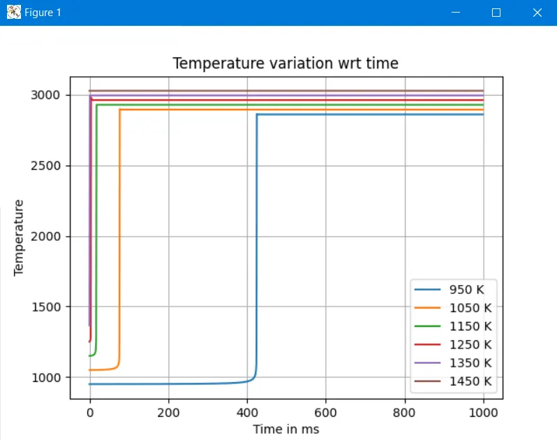

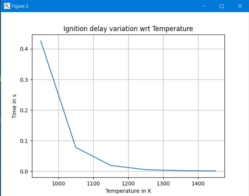
We can see as the temperature increases Ignition delay period decreases. Ignition delay is more sensitive to temperature increase as we can see the curve for temperature and Ignition delay plot is steeper than the pressure and Ignition delay plot.

PART II

Further, observe and print the rate of change of molar concentrations of the given elements "H2O, O2, OH" with respect to the time, (simulation time = 10 secs)

Explain the behaviour of the graph for 2 cases,

• When Temperature is 1000K and pressure 5 bar
• When Temperature is 500K and pressure 5 bar

''' 
PART II
Further, observe and print the rate of change of molar concentrations of the given elements
"H2O, O2, OH" with respect to the time, (simulation time = 10 secs)
Explain the behavior of the graph for 2 cases -->
1. When Temperature is 1000K and pressure 5 bar
2. When Temperature is 500K and pressure 5 bar
NOTE:
The command to extract mole fractions of a given 'species' is,
states.X[:,gas.species_index('species')])
'''
import numpy as nu
import matplotlib.pyplot as plt
import cantera as ct
import sys
T1=500
T2=1000
T = [T1,T2]
P=5*101325
gas = ct.Solution('gri30.xml')
for i in range(len(T)):
   if i==0:
      gas.TPX = T[i], P, {'CH4':1,'O2':2,'N2':7.52}
      # Creating reactor networks
      r=ct.IdealGasReactor(gas)
      sim=ct.ReactorNet([r])
      time=0.0
      # defining solution arrays
      states=ct.SolutionArray(gas, extra=['time_in_ms','t'])
      for n in range(1000):
         time += 1e-3 # 1 ms [Cantera chooses its own time step]
         sim.advance(time)
         states.append(r.thermo.state, time_in_ms=time*1e-3, t=time)
      # plot the molar concentrations
      plt.figure(1)
      plt.subplot(2,1,1)
      plt.plot(states.t,states.X[:,gas.species_index('H2O')])
      plt.xlabel('Time')
      plt.ylabel('concentration of H2O') 
      plt.legend(['500 K'])
      plt.figure(2)
      plt.subplot(2,1,1)
      plt.plot(states.t,states.X[:,gas.species_index('O2')])
      plt.xlabel('Time')
      plt.ylabel('concentration of O2') 
      plt.legend(['500 K'])
      plt.figure(3)
      plt.subplot(2,1,1)
      plt.plot(states.t,states.X[:,gas.species_index('OH')])
      plt.xlabel('Time')
      plt.ylabel('concentration of OH') 
      plt.legend(['500 K'])
   if i==1:
      gas.TPX = T[i], P, {'CH4':1,'O2':2,'N2':7.52}
      # Creating reactor networks
      r=ct.IdealGasReactor(gas)
      sim=ct.ReactorNet([r])
      time=0.0
      # defining solution arrays
      states=ct.SolutionArray(gas, extra=['time_in_ms','t'])
      for n in range(1000):
         time += 1e-3 # 1 ms [Cantera chooses its own time step]
         sim.advance(time)
         states.append(r.thermo.state, time_in_ms=time*1e-3, t=time)
      # plot the molar concentrations
      plt.figure(1)
      plt.subplot(2,1,2)
      plt.plot(states.t,states.X[:,gas.species_index('H2O')])
      plt.xlabel('Time')
      plt.ylabel('concentration of H2O') 
      plt.legend(['1000 K'])
      plt.figure(2)
      plt.subplot(2,1,2)
      plt.plot(states.t,states.X[:,gas.species_index('O2')])
      plt.xlabel('Time')
      plt.ylabel('concentration of O2') 
      plt.legend(['1000 K'])
      plt.figure(3)
      plt.subplot(2,1,2)
      plt.plot(states.t,states.X[:,gas.species_index('OH')])
      plt.xlabel('Time')
      plt.ylabel('concentration of OH') 
      plt.legend(['1000 K'])
plt.show()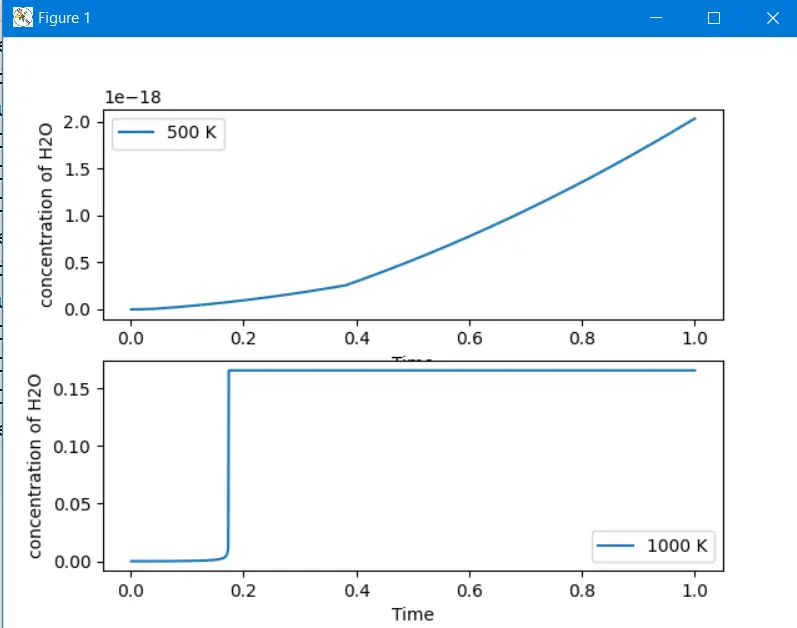

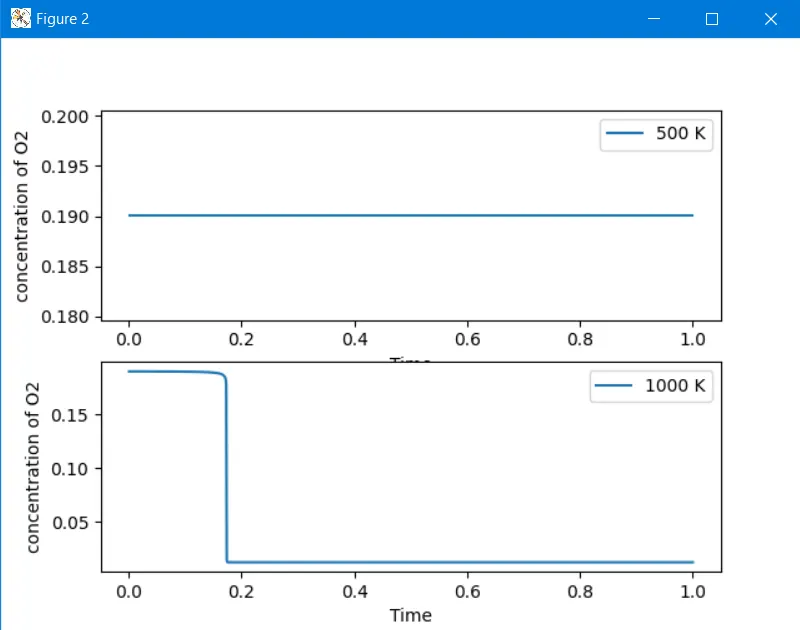
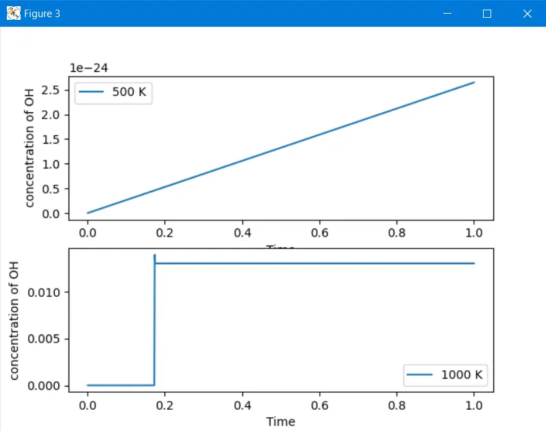
--> O2 concentration for 500 K case is not varying and is almost constant. The Ignition temperature for methane is around 700 K so at 500 K we will not see combustion take place. We infer from the H2O and OH concentration plot that chemical reactions are taking place and products are forming slowly, but the rate of chemical reaction is very low and it is not able to combust.

--> In the other case of 1000 K initial temperature we see an abrupt change in concentrations of species in very short time span. Combustion has taken place in the second case and products have formed.