Week 7 - Auto ignition using Cantera

Autoignition using Cantera

Aim:-

To find a variation of Auto Ignition time of Methane under various conditions, and observe the rate of change of molar concentrations of the given elements "H2O, O2, OH" with respect to the time.

Autoignition:-

Autoignition temperature is the lowest temperature at which it spontaneously ignites without an external source of ignition, such as a flame or spark. This temperature is required to supply the activation energy needed for combustion. The temperature at which a chemical ignites decreases as the pressure or Oxygen concentration increases. It is usually applied to a combustible fuel mixture.

Autoignition of Methane CH4:-

Autoignition temperatures for stoichiometric methane-air mixtures are around 870 K (600°C) at atmospheric pressure and decrease to 660 K (390°C) at 1100 bar ignition pressure.

Ignition delay:-

Ignition delay (ID) is defined as the time period required to raise the Temperature from the initial temperature(T) state to T(initial + 400K).

Auto Ignition time is the time when the temperature of the reactor is Initial Temperature plus 400K

`text(Time)_(text(ignition delay)) = text(Time)_(text(initial temperature + 400K))`

PART I :-

Use reactor network code to simulate the Auto Ignition Time for Methane under the following conditions,

simulation time = 10 secs => 10*1000 = 10000 milli sec

Procedure:-

1. Import the required modules, like numpy, matplotlib & cantera
2. Create gas class using solution template class in cantera.
3. Define initial conditions like temperature, pressure & mole fractions.
4. Creating a Reactor type in which Reaction takes place. ()IdealGasReactor.
5. Reaction network to calculate reactions
6. Create a Solution array to store the results computed by the Reactor network.
7. use for loop for a range of simulation time
8. Advance Time by 1 millisecond and run Reaction network.
9. store the solution values to the solution array.
10. calculate ignition delay time.
11. Repeat the process from step 4 for different initial Pressure, temperature values according to the case. using for loop
12. Plot the results.
13. Give conclusions.

====================================================

Case1:-

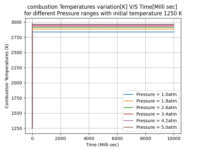
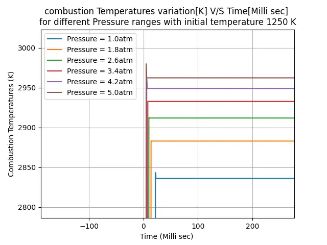
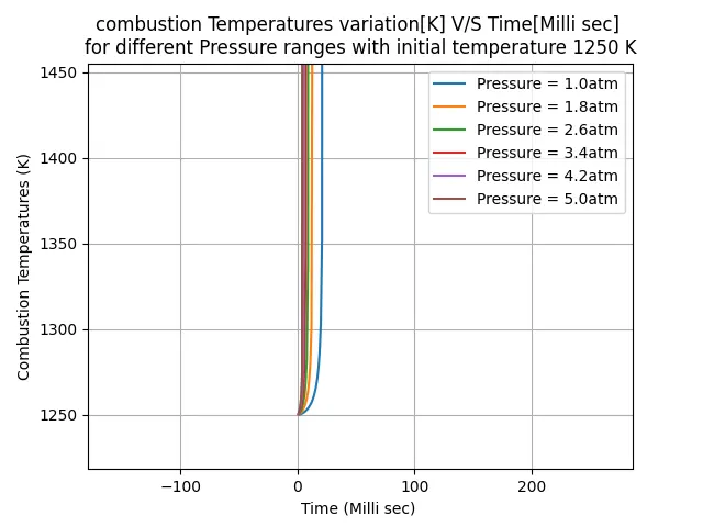
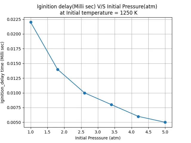
Plot the variation of Auto Ignition time of Methane with a constant temperature of 1250K and pressure varying from 1 to 5 atm.

`T_(text(initial)) = 1250K`

`P_(text(initial)) = 1-5 text( atm)`

Main Program:-

"""variation of Auto Ignition time of Methane with a constant temperature of 1250K
and pressure varying from 1 to 5 atm.
"""
# importing numpy, matplotlib, cantera moduels
import numpy as np
import matplotlib.pyplot as plt
import cantera as ct


gas = ct.Solution('gri30.xml')   # creating gas object using solution class template


sim_time = 10000     # simulation time = 10 seconds  = 10*1000 Milli sec
# Initial conditions
T_i = 1250  # constant temperature of 1250K
Pressure_i = np.linspace(101325, 5*101325, 6)   # pressure varying from 1 to 5 atm.

Iginition_delay = []

for P in Pressure_i:
	# assigning Temperature Pressure, Moles as attributes
	gas.TPX = T_i, P, {'CH4': 1, 'O2': 2, 'N2': 7.52}

	Reactor = ct.IdealGasReactor(gas)      # Creating a Reactor type in which Reaction takes place
	sim = ct.ReactorNet([Reactor])         # Reaction network to calculate reactions
	time = 0.0    # sarting time
	states = ct.SolutionArray(gas, extra=['time_in_ms', 't'])  # Sloution array to store Results
	C = 0

	for n in range(sim_time):
		time += 1e-3    # time increment
		sim.advance(time)   # simulation advances with time increment
		states.append(Reactor.thermo.state, time_in_ms=time*1e3, t=time)   # storing data

		if (states.T[n]-T_i) >= 400 and C == 0:
			Iginition_delay.append(time)    # finding Ignition delay
			C = C + 1
	# Plotting Results
	plt.figure(1)
	plt.plot(states.time_in_ms, states.T)
plt.xlabel("Time (Milli sec) ")
plt.ylabel("Combustion Temperatures (K)")
plt.legend(['Pressure = ' + str(P/101325) + 'atm' for P in Pressure_i])
plt.title('''combustion Temperatures variation[K] V/S Time[Milli sec] 
for different Pressure ranges with initial temperature 1250 K''')
plt.grid('on')

plt.figure(2)
plt.plot(Pressure_i/101325, Iginition_delay, marker='o')
plt.xlabel("Initial Presssure (atm)")
plt.ylabel("Iginition_delay time (Milli sec)")
plt.title("Iginition delay(Milli sec) V/S Initial Pressure(atm) \n at Initial temperature = 1250 K")
plt.grid('on')

print('S.No Initial Pressure(atm)     Iginition_delay[Milli sec]')
for i in range(len(Pressure_i)): print('  %d    %12.3f        %15.3f' % (i, Pressure_i[i], Iginition_delay[i]))
plt.show()

Plots:-

Result explanation:

• Autoignition temperatures for stoichiometric methane-air mixtures are around 870 K(600°C) at atmospheric pressure, it is the maximum autoignition temperature for methane. we given initial temperature as 1250K which is greater than the 870K i.e., all the above combustions don't need any external heat source for the combustion reaction.
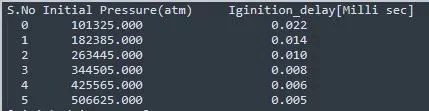
• As we fixed the initial Temperature and varied pressure from 1atm to 5atm ignition delay time reduced from 0.022millisec - 0.005millisec.

Conclusion:

• From plots and result table we can say that as the pressure increases at constant temperature Ignition delay gets decreased.

--------------------------------------------------------------------------------------------------

Case 2:-

Plot the variation of Auto Ignition time of Methane with a constant pressure of 5 atm and temperature varying from 950K to 1450K.

`P_(text(initial)) = 5 text( atm)`

`T_(text(initial)) = 950-1450K`

Main Program:-

"""variation of Auto Ignition time of Methane with a
constant pressure of 5 atm and temperature varying from 950K to 1450K.
"""
# importing numpy, matplotlib, cantera moduels
import numpy as np
import matplotlib.pyplot as plt
import cantera as ct


gas = ct.Solution('gri30.xml')   # creating gas object using solution class template


sim_time = 10000    # simulation time = 10 seconds  = 10*1000 Milli sec
# Initial conditions
P_i = 5 * 101325  # constant Pressure of 1250K
Temperature_i = np.linspace(950, 1450, 6)       # Temperature varying from 950K to 1450K.

Iginition_delay = []

for Temp in Temperature_i:
    # assigning Temperature Pressure, Moles as attributes
    gas.TPX = Temp, P_i, {'CH4': 1, 'O2': 2, 'N2': 7.52}   # initial conditions
    
    Reactor = ct.IdealGasReactor(gas)      # Creating a Reactor type in which Reaction takes place
    sim = ct.ReactorNet([Reactor])         # Reaction network to calculate reactions
    time = 0.0  # sarting time
    states = ct.SolutionArray(gas, extra=['time_in_ms', 't'])
    C = 0
    
    for n in range(sim_time):
        time += 1e-3  # time increment
        sim.advance(time)  # simulation advances with time increment
        states.append(Reactor.thermo.state, time_in_ms=time * 1e3, t=time)  # storing data

        if (states.T[n] - Temp) >= 400 and C == 0:
            Iginition_delay.append(time)  # finding Ignition delay
            C = C + 1
    # Plotting Results
    plt.figure(1)
    plt.plot(states.time_in_ms, states.T)
plt.xlabel("Time (Milli sec) ")
plt.ylabel("Combustion Temperatures (K)")
plt.legend(['Initial temp = ' + str(T) + '[K]' for T in Temperature_i])
plt.title('''combustion Temperatures[K] V/S Time [Milli sec] 
for different Initial Temperature's with constant initial pressure = 5 atm''')
plt.grid('on')

plt.figure(2)
plt.plot(Temperature_i, Iginition_delay, marker='o')
plt.xlabel("Initial Temperature's [K]")
plt.ylabel("Iginition_delay time (Milli sec)")
plt.title("Iginition delay V/S Initial Temperature ")
plt.grid('on')

print('S.No Initial Temperature[K]     Iginition_delay[Milli sec]')
for i in range(len(Temperature_i)): print('  %d    %12.3f        %15.3f' % (i, Temperature_i[i], Iginition_delay[i]))
plt.show()

Plots:-

Result explanation:

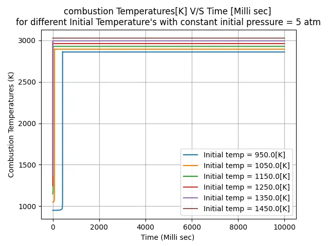
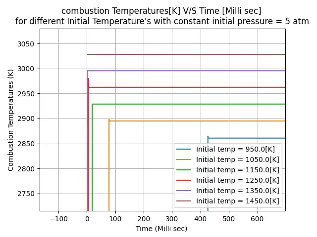
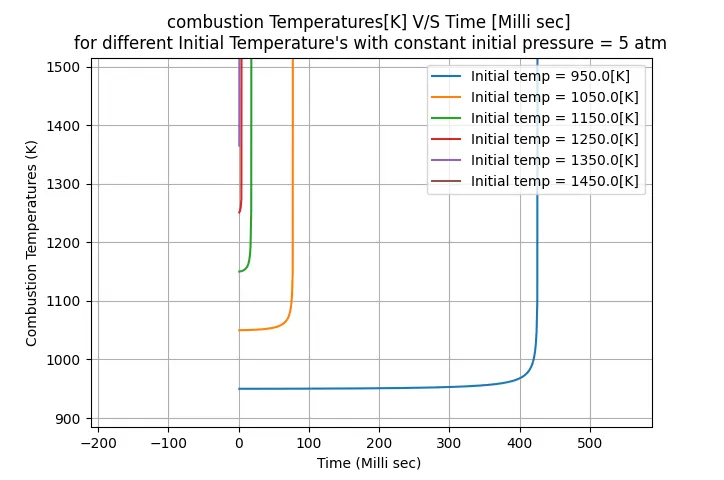
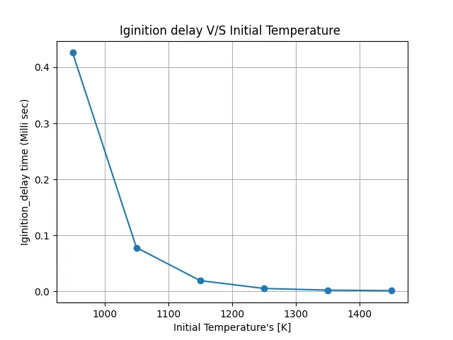
• Autoignition temperatures for stoichiometric methane-air mixtures are around 870 K(600°C) at atmospheric pressure, it is the maximum autoignition temperature for methane. we given initial temperature ranges from 950K - 1450K which is greater than the 870K i.e., all the above combustions don't need any external heat source for the combustion reaction.
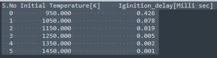
• As we fixed the initial Pressure as 5atm and varied Temperature from 950K - 1450K ignition delay time reduced from 0.426millisec - 0.001millisec.

Conclusion:

• From plots and result table we can say that as the Temperature increases at constant Pressure Ignition delay gets decreases drastically.

--------------------------------------------------------------------------------------------------

PART II:-

Observe the rate of change of molar concentrations of the given elements "H2O, O2, OH" with respect to the time Simulation time.

Explain the behavior of the graph for 2 cases,

• When Temperature is 1000K and pressure 5 bar
• When Temperature is 500K and pressure 5 bar

`P_(text(initial)) = 5 text( atm)`

`T_(text(initial)) = 500K , 1000K`

Main Program:-

"""variation of Auto Ignition time of Methane with a
constant pressure of 5 atm and temperature varying from 950K to 1450K.
"""
# importing numpy, matplotlib, Cantera, modules
import matplotlib.pyplot as plt
import cantera as ct


def ploting(x, y, element, temp):
    plt.figure(figsize=(12, 6))
    plt.plot(x, y)
    plt.xlabel("Time (Milli sec) ")
    plt.ylabel("Molar concentration")
    plt.legend(['Molar concentration of' + element])
    plt.title("Molar concentration V/S Time [Milli sec] plot for methane combustion \n for Initial Temperature =" + str(temp) + " with constant initial pressure = 5 atm")
    plt.grid('on')
    plt.savefig(("fig" + str(temp) + element + ".jpg"))


gas = ct.Solution('gri30.xml')   # creating gas object using solution class template


sim_time = 10000    # simulation time = 10 seconds  = 10*1000 Milli sec
# Initial conditions
P_i = 5 * 101325              # constant Pressure of 1250K
Temperature_i = [500, 1000]   # Temperature varying from 950K to 1450K.
Iginition_delay = []
Elements = ['H2O', 'O2', 'OH']
Element_concentration = []
i = 1

for Temp in Temperature_i:
    # assigning Temperature Pressure, Moles as attributes
    gas.TPX = Temp, P_i, {'CH4': 1, 'O2': 2, 'N2': 7.52}  # initial conditions

    Reactor = ct.IdealGasReactor(gas)      # Creating a Reactor type in which Reaction takes place
    sim = ct.ReactorNet([Reactor])         # Reaction network to calculate reactions
    time = 0.0  # starting time
    states = ct.SolutionArray(gas, extra=['time_in_ms', 't'])
    C = 0

    for n in range(sim_time):
        time += 1e-3  # time increment
        sim.advance(time)  # simulation advances with time increment
        states.append(Reactor.thermo.state, time_in_ms=time * 1e3, t=time)  # storing data

        if (states.T[n] - Temp) >= 400 and C == 0:
            Iginition_delay.append(time)  # finding Ignition delay
            C = C + 1
    H2O_concentration = states.X[:, gas.species_index('H2O')]
    O2_concentration = states.X[:, gas.species_index('O2')]
    OH_concentration = states.X[:, gas.species_index('OH')]

    plt.figure(i); i = i + 1
    ploting(states.time_in_ms, H2O_concentration, 'H2O', Temp)
    plt.figure(i); i = i + 1
    ploting(states.time_in_ms, O2_concentration, 'O2', Temp)
    plt.figure(i); i = i + 1
    ploting(states.time_in_ms, OH_concentration, 'OH', Temp)
plt.show()

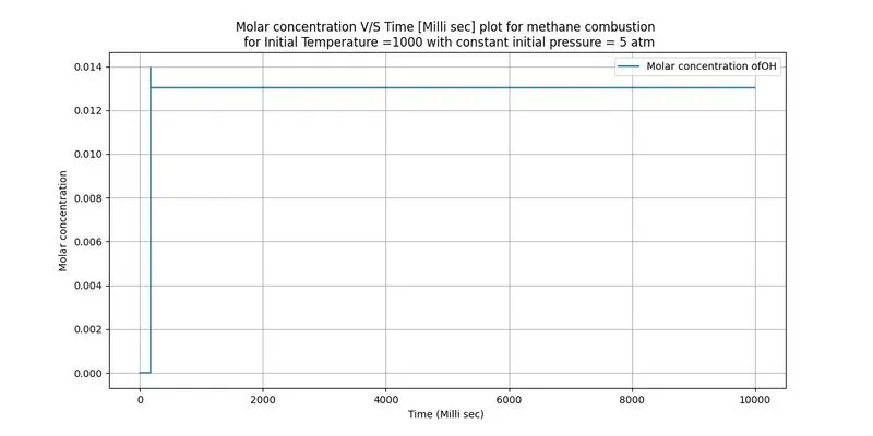
Plots:-

T = 1000K > T_auto

fig 1

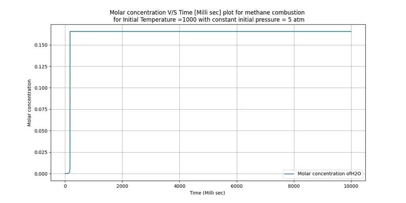
fig 2

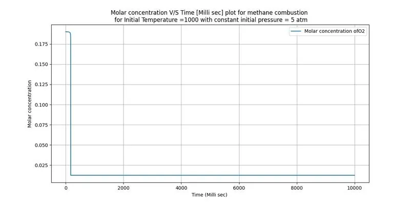
fig 3

• `CH_4 + 2(O_2+3.76N_2) = CO_2 + 2H_2O + 7.52N_2`
• from fig1, we can observe that H2O Molar concentration is constant initially up to Ignition delay time, after ignition delay time Molar concentration of H2O increases rapidly reaches the maximum point from that point concentration maintained at a constant level.
• from fig2, we can observe that O2 Molar concentration is constant initially up to Ignition delay time, after ignition delay time Molar concentration of O2 decreases rapidly reaches the minimum point from that point concentration maintained at a constant level.
• from fig3, we can observe that OH Molar concentration is constant initially up to Ignition delay time, after ignition delay time Molar concentration of H2O increases rapidly reaches the maximum point but is no longer stable at that point within few mi9lli seconds its concentration decreases slightly from that point concentration maintained at a constant level.

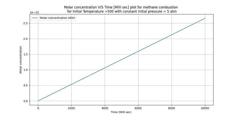
T = 500 K < T_auto

fig 4

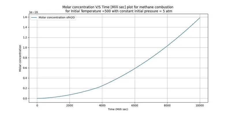
fig 5

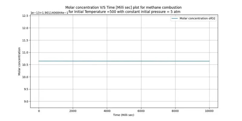
fig 6

Conclusion:-

• We can observe that all fig 4,6 plots molecular concentration order les than 1e-15 & O2 concentration fairly maintained constant it clearly showing that combustion was not taken in that reactor. by seeing the initial temperature value we can clearly say that combustion reaction will not take place at that temperature because we gave the initial temperature as 500K which is less than least auto-ignition temperature oh methane(660K) at 1100 bar.
• in fig 4, 6:- we can notice that there is a slight increase in the H2O, OH concentration in the order of 1e-16, 1e-23 respectively these values are absolutely negligible but where do these products come from ?.
• This happened due to the initial temperature of 500K maintained for sufficient time to take cause Oxidation reaction.
• As the two graphs are growing continuously if we wait for a long enough time means really long time it may have some effect.
• By seeing fig 5, we will think that O2 concentration is maintained constantly because combustion has not taken place but OH, H2O products are formed from O it means O2 has been decreasing along with an increase in OH, H2O concentration. i.e., in the above statement, I concluded that if we really wait for a very very long enough time reactants will convert into products due to oxidation of fuel.