Week 7 - Auto ignition using Cantera

AUTO IGNITION USING CANTERA

AIM: to simulate the Auto Ignition Time for Methane and observe and print the rate of change of molar concentrations.

OBJECTIVE:

PART I

Use the same reactor network code as shown in the video to simulate the Auto Ignition Time for Methane under the following conditions, (simulation time = 10 secs)

• Plot the variation of Auto Ignition time of Methane with a constant temperature of 1250K and pressure varying from 1 to 5 atm.
• Plot the variation of Auto Ignition time of Methane with a constant pressure of 5 atm and temperature varying from 950K to 1450K.

PART II

Further, observe and print the rate of change of molar concentrations of the given elements "H2O, O2, OH" with respect to the time, (simulation time = 10 secs)

Explain the behavior of the graph for 2 cases,

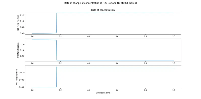
• When Temperature is 1000K and pressure 5 bar
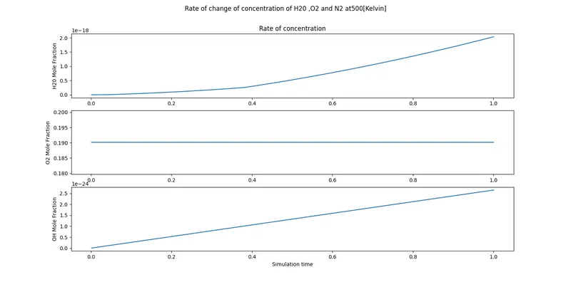
• When Temperature is 500K and pressure 5 bar

THEORY

Auto Ignition Temperature of a mixture is the lowest temperature at which the mixture would ignite. The Air-Fuel mixture does not burn immediately and takes time for the reaction to take place. Hence the Auto Ignition time is the time required for the chemical reaction to take place.

And Ignition delay is the time interval between the start of injection and the start of combustion. This delay period consists of (a) physical delay, wherein atomization, vaporization, and mixing of air-fuel occur, and

(b) of chemical delay attributed to pre-combustion reactions. Physical and chemical delays occur simultaneously. To reduce NOx, the method adopted in modern engines is to reduce the ignition delay.

`Time_(Ignition Delay)=Time_(Initial Temperature+400K)`

The stoichiometric combustion of Methane is considered in this case. The combustion equation for methane:

`CH_4+2O_2+7.56N_2 rightarrow CO_2+2H_2O+7.56N_2`

CODE AND SOLUTION:

CASE 1:

(a) In this case we are considering the constant temperature of 1250K and pressure varying from 1 to 5 ATM.

import sys
import cantera as ct
import matplotlib.pyplot as plt
import numpy as np

gas = ct.Solution('gri30.xml')
p_start = ct.one_atm
p_end = ct.one_atm*5
n = 5
pr = np.linspace(p_start,p_end,n) 
ignition_delay=[]

for i in range(1,6):

	P=ct.one_atm*i 
	T=1250 
	gas.TPX=T,P,{'CH4':1,'O2':2,'N2':7.52}
	r=ct.IdealGasReactor(gas)
	sim=ct.ReactorNet([r])
	time=0
	sim_time=10*100
	states=ct.SolutionArray(gas,extra=['time_in_ms','t'])
	T_old=T


	for j in range(sim_time+1):
		time+=1e-3
		sim.advance(time) 
		states.append(r.thermo.state,time_in_ms=time*1e-3,t=time)	

		T_new = states.T
		T_new = T_new[j-1]

		if (T_new-T_old)>=400:
			ignition_delay.append(time)

		T_old = states.T
		T_old = T_old[j-1]

		
	plt.subplot(2,1,1)
	plt.plot(states.t,states.T)
	plt.xlabel('Simulation time (ms)')
	plt.ylabel('Temprature(k)')
	plt.legend(['Pressure -'+str(P)+'[atm]'for P in pr])

plt.subplot(2,1,2)
plt.plot((pr/101325),ignition_delay,'-o')
plt.xlabel('Pressure')
plt.ylabel('ignition_delay')	
plt.show()

RESULT

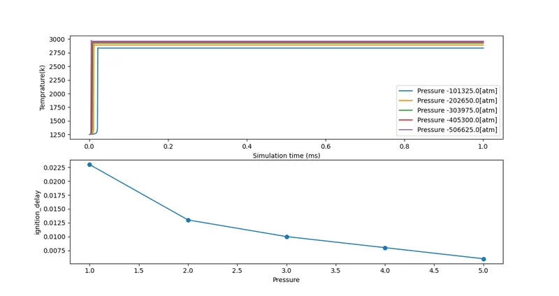
In this case, we see that the plot of Methane under the variation of Pressure and Temperature i.e, temperature increases proportionally to the pressure. Initially, pressure needs more time to auto-ignite producing low temperature.

The second Plot defines Ignition-delay, where pressure increases as ignition delay decrease because according to Ideal gas, the equation pressure is directly proportional to the temperature and the Initial temperature is high ignition delay is low.

(b) In this case we are considering the constant pressure of 5ATM and temperature is varying between 950K and 1450K.

import sys
import cantera as ct
import matplotlib.pyplot as plt
import numpy as np

gas = ct.Solution('gri30.xml')
T_start=950 
T_end=1450 
n=10
Temp=np.linspace(T_start,T_end,n)
ignition_delay=[]

for i in range(len(Temp)):

	P=ct.one_atm*5 
	gas.TPX=Temp[i],P,{'CH4':1,'O2':2,'N2':7.52}
	r=ct.IdealGasReactor(gas)
	sim=ct.ReactorNet([r])
	time=0
	states=ct.SolutionArray(gas,extra=['time_in_ms','t'])
	sim_time=10*100
	T_old = Temp[i]	
		
	for j in range (sim_time+1):
		time+=1e-3
		sim.advance(time)
		states.append(r.thermo.state,time_in_ms = 1e-3*time, t= time)

		T_new = states.T
		T_new = T_new[j-1]

		if ((T_new-T_old)>=400):
			ignition_delay.append(time)

		T_old = states.T
		T_old = T_old[j-1]

	plt.subplot(2,1,1)
	plt.plot(states.t,states.T)
plt.xlabel('Simulation time(ms)')
plt.ylabel('Temperature(k)')
plt.legend(['Intial_T ='+str(T) +'[k]' for T in Temp])

plt.subplot(2,1,2)
plt.plot(Temp,ignition_delay,'-o')
plt.xlabel('Intial temperature (k)')
plt.ylabel('ignition_delay')
plt.show()

RESULT

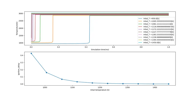
In the above plot, we can see that Methane under the variation of temperature and constant pressure, for temperature variation: The temperature increases as ignition delay decreases. Initially, the temperature needs more time to auto-ignite, if the temperature is low, ignition delay high. As compared to the pressure the ignition delay is faster because of the temperature high. It may help with the auto-ignition.

CASE 2:

Calculating rate of change of concentration for species H2O O2 and OH

import numpy as np
import cantera as ct
import sys
import matplotlib.pyplot as plt

Temp = [1000,500]

for T in Temp:
	gas = ct.Solution('gri30.xml')
	P = ct.one_atm*5
	gas.TPX = T,P,{'CH4':1,'O2':2,'N2':7.52}
	r = ct.IdealGasReactor(gas)
	sim = ct.ReactorNet([r])
	time = 0
	states = ct.SolutionArray(gas,extra=['time_in_ms','t'])
	sim_time = 10*100
	for i in range(sim_time+1):
		time+=1e-3
		sim.advance(time)
		states.append(r.thermo.state,time_in_ms=time*1e-3,t=time)

	# H2O Plot 
	plt.subplot(3,1,1)
	plt.plot(states.t,states.X[:,gas.species_index('H2O')])
	plt.ylabel('H20 Mole Fraction')
	plt.title('Rate of concentration')

	
	# O2 plot 
	plt.subplot(3,1,2)
	plt.plot(states.t,states.X[:,gas.species_index('O2')])
	plt.ylabel('O2 Mole Fraction')
	

	# OH plot 
	plt.subplot(3,1,3)
	plt.plot(states.t,states.X[:,gas.species_index('OH')])
	plt.xlabel('Simulation time')
	plt.ylabel('OH Mole Fraction')
	plt.suptitle('Rate of change of concentration of H20 ,O2 and N2 at' + str(T) + '[Kelvin]')
	plt.show()

RESULT

When Temperature is 1000K and pressures 5 bar we calculate the molar fraction of products species using Cantera

In the below figure we can see the rate of the molar fraction of H2O, O2, and OH at 1000K.

As we see in the first plot: H2O is respectively very less before auto-ignition. As we know that the Reaction of Methane and Air forms a product of H2O and its starting very little after ignition takes place and increases gradually and at some point it stable this is called equilibrium chemistry.

In the second plot, the mole fraction of O2 respectively decreases because when air reacts with the fuel it gets oxidized.

The third plot tells the mole fraction of OH is respectively less before auto-ignition.

When Temperature is 500K and pressure 5 bar, the rate mole fraction is less as compared to the 1000K because the initial temperature was very low. In the first plot, we see that Auto-ignition takes place very slowly and in the second plot O2 is not completely automize because the initial temperature was very low.