Auto ignition using Cantera

Introduction

• A mixture requires the right conditions to burn. Everything should be correct – Temperature, Pressure, Fuel-Air mixture, etc.
• Auto-Ignition is the lowest temperature at which the mixture combusts. Before Auto-Ignition, there exists a period called ignition delay, that is the time before which combustion occurs. (order of micro seconds) Calculating this delay, and how it varies with different parameters like starting temperature, pressure, etc. can be very useful for combustion applications.

Aim

Part 1

• Plot the variation of Auto Ignition time of Methane with a constant temperature of 1250K and pressure varying from 1 to 5 atm.
• Plot the variation of Auto Ignition time of Methane with a constant pressure of 5 atm and temperature varying from 950K to 1450K.

Part 2

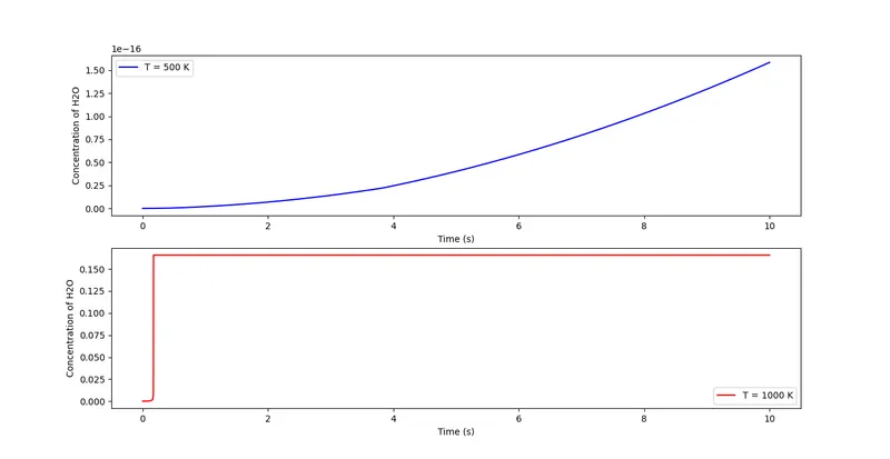
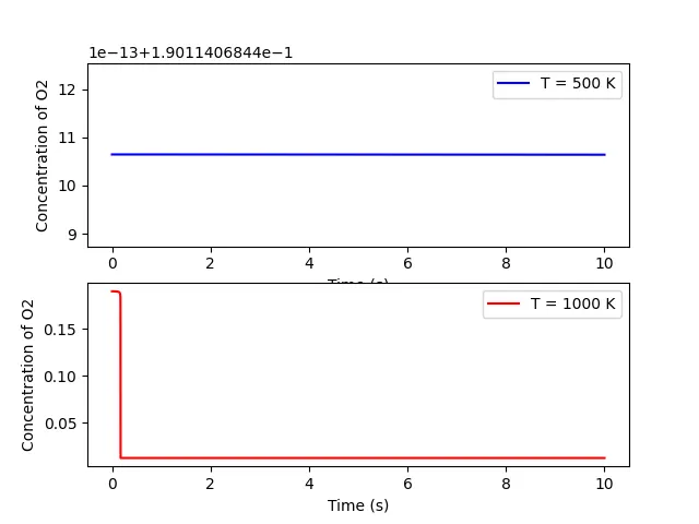
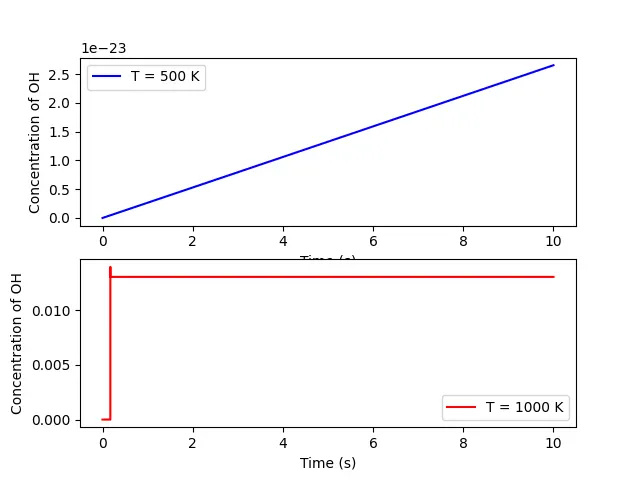
Observe and print the rate of change of molar concentrations of the given elements "H2O, O2, OH" with respect to the time, (simulation time = 10 secs)

Explain the behavior of the graph for 2 cases:

• When Temperature is 1000K and pressure 5 bar
• When Temperature is 500K and pressure 5 bar

Results

A python code is written, and Cantera is used for the execution of the study.

Part 1

1.1 Plot the variation of Auto Ignition time of Methane with a constant temperature of 1250K and pressure varying from 1 to 5 atm.

Code:

import sys
import numpy as np 
import cantera as ct
import matplotlib.pyplot as plt
gas = ct.Solution('gri30.xml')

#creating initial temperature and pressure conditions
T = 1250
P = [1,2,3,4,5]

ignition_delay = [] #creating an empty array that stores the time at which ignition begins

for i in range(len(P)):
	
	#create gas object
	gas.TPX = T,P[i]*101325,{'CH4':1,'O2':2,'N2':7.52}

	#create reactor object that takes in the gas object
	r = ct.IdealGasReactor(gas)
	
	sim = ct.ReactorNet([r])

	time = 0.0
	states = ct.SolutionArray(gas, extra = ['time_in_ms','t'])

	for n in range(10000):
		time += 1e-3
		sim.advance(time)
		states.append(r.thermo.state,time_in_ms = time*1e3, t = time)

	for j in range (len(states.T)):
		if states[j].T >= (1250+400):
			ignition_delay.append(states.time_in_ms[j])

			break


plt.plot(P,ignition_delay)
plt.xlabel('Pressure (bar)')
plt.ylabel('ignition delay (ms)')
plt.show()


'''
plt.plot(states.T)
plt.show()
'''

Result:

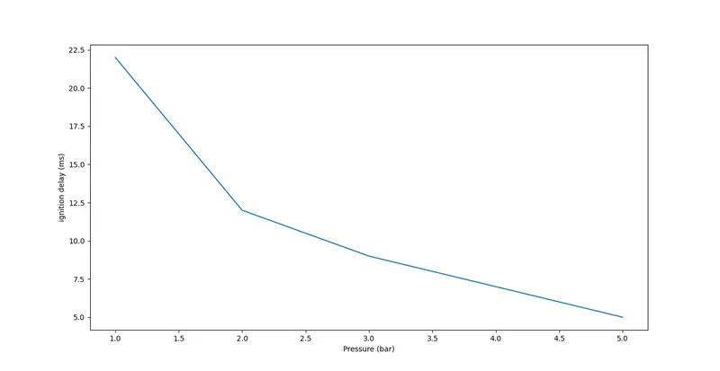
Thus, increasing the pressure reducing the ignition delay in this case.

1.2 Plot the variation of Auto Ignition time of Methane with a constant pressure of 5 atm and temperature varying from 950K to 1450K.

Code:

import sys
import numpy as np 
import cantera as ct
import matplotlib.pyplot as plt
gas = ct.Solution('gri30.xml')

T = np.linspace(950,1450,10)
P = 5*101325


ignition_delay = []
#create gas object
for i in range(len(T)):
	
	gas.TPX = T[i],P,{'CH4':1,'O2':2,'N2':7.52}

	#create reactor object that takes in the gas object
	r = ct.IdealGasReactor(gas)
	#help(r)
	sim = ct.ReactorNet([r])

	time = 0.0
	states = ct.SolutionArray(gas, extra = ['time_in_ms','t'])

	for n in range(10000):
		time += 1e-3
		sim.advance(time)
		states.append(r.thermo.state,time_in_ms = time*1e3, t = time)

	for j in range (len(states.T)):
		if states[j].T >= (1250+400):
			ignition_delay.append(states.time_in_ms[j])

			break


plt.plot(T,ignition_delay)
plt.xlabel('Temperature (K) ')
plt.ylabel('ignition delay (ms)')
plt.show()


'''
plt.plot(states.T)
plt.show()
'''

Result:

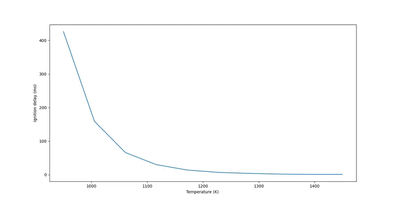
Therefore, increasing the initial pressure reduces the ignition delay as well, similar to pressure.

Part 2

2.1 Observe and print the rate of change of molar concentrations of the given elements "H2O, O2, OH" with respect to the time, (simulation time = 10 secs)

Code:

import sys
import numpy as np 
import cantera as ct
import matplotlib.pyplot as plt
gas = ct.Solution('gri30.xml')

T = [500,1000]
P = 5*101325



#create gas object
for i in range(len(T)):
	
	gas.TPX = T[i],P,{'CH4':1,'O2':2,'N2':7.52}

	#create reactor object that takes in the gas object
	r = ct.IdealGasReactor(gas)
	#help(r)
	sim = ct.ReactorNet([r])

	time = 0.0
	states500 = ct.SolutionArray(gas, extra = ['time_in_ms','t'])
	states1000 = ct.SolutionArray(gas, extra = ['time_in_ms','t'])


	if i == 0:
		for n in range(10000):
			time+= 1e-3
			sim.advance(time)
			states500.append(r.thermo.state,time_in_ms = time*1e3, t = time)
	plt.figure(1)
	plt.subplot(2,1,1)
	plt.plot(states500.t,states500.X[:,gas.species_index('H2O')],color = 'blue')
	plt.xlabel('Time (s)')
	plt.ylabel('Concentration of H2O')
	plt.legend(['T = 500 K'])

	plt.figure(2)
	plt.subplot(2,1,1)
	plt.plot(states500.t,states500.X[:,gas.species_index('O2')],color = 'blue')
	plt.xlabel('Time (s)')
	plt.ylabel('Concentration of O2')
	plt.legend(['T = 500 K'])

	plt.figure(3)
	plt.subplot(2,1,1)
	plt.plot(states500.t,states500.X[:,gas.species_index('OH')],color = 'blue')
	plt.xlabel('Time (s)')
	plt.ylabel('Concentration of OH')
	plt.legend(['T = 500 K'])

	if i == 1:
		for n in range(10000):
			time+= 1e-3
			sim.advance(time)
			states1000.append(r.thermo.state,time_in_ms = time*1e3, t = time)
		
	plt.figure(1)
	plt.subplot(2,1,2)
	plt.plot(states1000.t,states1000.X[:,gas.species_index('H2O')],color = 'red')
	plt.xlabel('Time (s)')
	plt.ylabel('Concentration of H2O')
	plt.legend(['T = 1000 K'])

	plt.figure(2)
	plt.subplot(2,1,2)
	plt.plot(states1000.t,states1000.X[:,gas.species_index('O2')],color = 'red')
	plt.xlabel('Time (s)')
	plt.ylabel('Concentration of O2')
	plt.legend(['T = 1000 K'])

	plt.figure(3)
	plt.subplot(2,1,2)
	plt.plot(states1000.t,states1000.X[:,gas.species_index('OH')],color = 'red')
	plt.xlabel('Time (s)')
	plt.ylabel('Concentration of OH')
	plt.legend(['T = 1000 K'])



plt.show()

Result:

H2O

O2

OH

Discussion

In this study, for part 1, it can be observed that with an increase in initial temperature and initial pressure, there is a decrease in ignition delay time. Thus, selecting a higher temperature or pressure initally is beneficial to increase the speed of combustion.

In part 2, the concentrations of some products and reactants were observed as they varied during the combustion time. When the temperature was 500K, it was observed that the concentration of O2 remained constant throughout, (even though an increase in H2O's concentration was observed), thus indicating that complete combustion has not taken place at 500 K.

At 1000 K however, for OH and H2O, a sudden increase in the concentration was observed (indicating combustion occuring after an intial delay), and then the concentration remained constant. The opposite was observed for O2, and this is expected as the concentration of O2 is supposed to decrease during the combustion process.