Week 6 - Multivariate Newton Rhapson Solver

The following set of ODEs are solved using Euler backward differencing method for time discretization and multivariate Newton Raphson technique to solve each time-step in iterative scheme.

`(dy_1)/(dt) = -0.04*y_1 + 10^4*y_2*y_3`
`(dy_2)/(dt) = 0.04*y_1 - 10^4*y_2*y_3 - 3*10^7*y_2^2`
`(dy_3)/(dt) = 3*10^7*y_2^2`

Initial conditions for [y1,y2,y3] at t0 is given as [1.0, 0.0, 0.0]

Approach:

The differential equations are converted to algrebraic equations using Euler backwards scheme that uses first order Taylor approximation such as

`y_1^n = y_1^(n-1) + h * (dy_1)/(dt) = y_1^(n-1) + h * (-0.04*y_1 + 10^4*y_2*y_3)^n`
`y_2^n = y_2^(n-1) + h * (dy_2)/(dt) = y_2^(n-1) + h * (0.04*y_1 - 10^4*y_2*y_3 - 3 * 10^7 * y_2^2)^n`
`y_3^n = y_3^(n-1) + h * (dy_3)/(dt) = y_3^(n-1) + h * (3*10^7*y_2^2)^n`

where, h -> time-step size that defines the difference between the time-steps 'n' and 'n-1'. These set of equations are solved for prescribed amount of time or until they reach nearly steady state. In this case, the equations are solved from initial time of 0[s] to 10[mins] using different values for h.

Since the set of equations described above are coupled to each other, the values of `y_1, y_2 and y_3` have to be approximated using a numerical scheme such as Gauss Jacobi or Gauss Siedel for each time-step. In this case, multivariate Newton-Raphson technique is used. For applying this scheme, the equations are rearranged to forms functions f1, f2 and f3 in the form of `f(y1, y2, y3) = 0` which can be solved using Newton-Raphson technique

`f_1 = y_1^(n-1) + h * (-0.04*y_1 + 10^4*y_2*y_3)^n - y_1^n = 0`
`f_2 = y_2^(n-1) + h * (0.04*y_1 - 10^4*y_2*y_3 - 3 * 10^7 *y_2^2)^n - y_2^n = 0`
`f_3 = y_3^(n-1) + h * (3*10^7*y_2^2)^n - y_3^n = 0`

Then the set of functions are solved for y using the iterative equation,

`y = y_(old) - alpha*J^-1*F`

where, `y` -> vector containing all the y values `y = [[y_1, y_2, y_3]]^T`

`y_(old)` -> vector containing y values from previous iteration

`F` -> vector of values estimated by the functions f1, f2 and f3 `F = [[f1,f2,f3]]^T`

`alpha` -> under-relaxation factor

`J` -> Jacobian matrix of size `(size(F) xx size(y))` that describes the first order derivatives of all functions in F with respect to all variables in y

`J = [[(delf_1)/(dely_1), (delf_1)/(dely_2), (delf_1)/(dely_3)],[(delf_2)/(dely_1), (delf_2)/(dely_2), (delf_2)/(dely_3)],[(delf_3)/(dely_1), (delf_3)/(dely_2), (delf_3)/(dely_3)]]`

The iterative equation is solved for multiple iterations until the difference between `y` and `y_(old)` are negligible, meaning the solution converged for the time-step.

Code:

A python program is written to solve the above described set of equations using backward Euler for time-step progressing and multivariate Newton-Raphson for iterative scheme. A function F is written that takes in y_old, y and dt values and returns the Fy vector containing the values of functions f1, f2 and f3 based on the algebraic equations for the functions. J function is written to take in the values of vector Fy, y_old, y and dt values to calculate the jacobian matrix with first order derivatives for the functions using numerical differentiation. Fy vector is converted to matrix Fy_stack of size(J) by stacking the F vectors horizontally. With small increments to individual y value, one vector is created for each y variable. Fy vectors with modified y vectors are calculated for each y variable and stacked horizontally to get a matrix Fdy of size(J). J is finally calculated using matrix operations by subtratring Fdy and Fy and dividing it by the increment value. This provides the numerical first order derivative of all functions with respect to y variables in Jacobian matrix form. A set of time-step size values are taken for analysis -> [0.1, 1.0, 10.0, 100.0]. For each value of dt, a solution is derived for y vector in the time frame of 0 to 10 mins. Total number of iterations and final y values are kept track of for each dt solution. Average number of iterations for each time-step is calculated for all values of dt. For each time-step value obtained using the time-step size value, residual value is reset to a large number so iterations would kick off. y values are kept track of for each time-step to be plotted against time. y_old vector is updated for each time-step to the values of y at previous time-step. A iterative loop is triggered for each time-step when residual is larger than a prescribed convergence criteria. Fy vector is calculated using F() function. Jacobian matrix is obtained using the J() function and it's inverse is obtained using the inv() method in numpy.linalg library. For each iteration, Newton-Raphson equation is solved to get a new set of y values. Residuals are updated and re-iterated until convergence is reached for time-step. Results are plotted for "y vs t" at the end of dt option. Results of "final y vs dt" and "average iterations vs dt" are plotted at the end of all simulations.

program:

'''
Solve a set of ODEs using multivariate Newton Raphson method and Backward Euler scheme
(dy_1)/(dt) = -0.04*y_1 + 10^4*y_2*y_3
(dy_2)/(dt) = 0.04*y_1 - 10^4*y_2*y_3 - 3*10^7*y_2^2
(dy_3)/(dt) = 3*10^7*y_2^2
[y1,y2,y3] at t0 = [1.0, 0.0, 0.0]

f_1 = y_1^(n-1) + h * (-0.04*y_1 + 10^4*y_2*y3)^n - y_1^n = 0
f_2 = y_2^(n-1) + h * (0.04*y_1 - 10^4*y_2*y_3 - 3 * 10^7 * y_2^2)^n - y_2^n = 0
f_3 = y_3^(n-1) + h * (3*10^7*y_2^2)^n - y_3^n = 0
'''
import numpy as np
import matplotlib.pyplot as plt

# constants
t0 = 0.0									# Intial time
tmax = 10.0*60								# final time
dt_arr = [0.1, 1.0, 10.0, 100.0]			# set of time-step sizes to be used
y0 = [1.0, 0.0, 0.0]						# Initial condition for y1,y2,y3 at t0
alpha = 1									# under relaxation factor
dy = 1e-6									# increment value used for numerical differentiation of F
tol = 1e-6									# convergence criteria
y_final = np.zeros((len(dt_arr),3))			# result array for final value of y
avg_iter = np.zeros((len(dt_arr)))			# result array to store average number of iterations for each dt


def F(y_old,y,dt):
	# Calculate Fy vector using the functions f1, f2 and f2 definition
	f1 = y_old[0] + dt * (-0.04*y[0] + pow(10,4)*y[1]*y[2]) - y[0]
	f2 = y_old[1] + dt * (0.04*y[0] - pow(10,4)*y[1]*y[2] - 3*pow(10,7)*pow(y[1],2)) - y[1]
	f3 = y_old[2] + dt * (3*pow(10,7)*pow(y[1],2)) - y[2]
	Fy = np.array([f1,f2,f3]).reshape(3,1)
	return Fy


def J(Fy,y_old,y,dt):
	# Calculate jacobian matrix using numerical differentiation
	Fy_stack = np.hstack((Fy,Fy,Fy))

	# Incremented y vectors for numerical differentiation	
	y_dy1 = y.copy()
	y_dy2 = y.copy()
	y_dy3 = y.copy()
	y_dy1[0] = y[0] + dy
	y_dy2[1] = y[1] + dy
	y_dy3[2] = y[2] + dy

	# F vectors based on incremented y vectors
	Fdy1 = F(y_old,y_dy1,dt)
	Fdy2 = F(y_old,y_dy2,dt)
	Fdy3 = F(y_old,y_dy3,dt)
	Fdy = np.hstack((Fdy1,Fdy2,Fdy3))

	# calculate and return jacobian
	J = ( Fdy - Fy_stack ) / dy
	return J

for j in range(len(dt_arr)):
	# loop over dt options provided

	dt = dt_arr[j]
	t_arr = np.arange(t0,tmax+dt,dt)									# time array to hold the time values
	y_arr = np.zeros((len(t_arr),3))									# y array to hold y values at different time-steps
	y_old = np.array(y0).reshape(3,1)									# y vector at previous time-step
	y = y_old.copy()													# y vector at current time-step
	y_arr[0] = y0[:]													# update y array with initial condition
	tot_iter = 0														# total iteration counter for each dt option

	for i in range(1,len(t_arr)):
		# loop over time values in time array

		t = t_arr[i]
		iter_ = 0														# iteration counter for each time-step
		err = 1e6 														# initialize residual/error to large value in each time-step
		#print("time: ",t)
		#print("\t"*4+"y0,"+"\t"*5+"y1,"+"\t"*5+"y2")

		while err > tol:
			# Newton-Raphson iterative loop

			Fy = F(y_old,y,dt)
			J_mat = J(Fy,y_old,y,dt)
			y_new = y - alpha * (np.linalg.inv(J_mat) @ Fy)
			err = np.max(np.abs(y_new - y))
			y = y_new.copy()
			iter_ += 1
			#print("iteration ",iter_, ": ", y[0,0], y[1,0], y[2,0])

			if iter_ > 1000:
				# break iterations if max limit is reached
				print("time",t, ": Solution did not converged")
				break

		# update y array, y_old vector and total iteration counter
		y_arr[i] = y[:,0]
		y_old = y.copy()
		tot_iter += iter_

	# Update final values of y for each dt option and calcualte average iterations
	y_final[j] = y[:,0]
	avg_iter[j] = tot_iter/len(t_arr)

	# plot y vs time for each dt option
	plt.figure(j+1)
	plt.plot(t_arr,y_arr)
	plt.grid()
	plt.xlabel("time [s]")
	plt.ylabel("y")
	plt.title("y vs time, dt =%0.2f" %dt)
	plt.legend(["y1","y2","y3"])

# plot final y for each dt option
plt.figure(len(dt_arr)+1)
plt.semilogx(dt_arr,y_final)
plt.grid()
plt.xlabel("dt [s]")
plt.ylabel("y_final")
plt.title("y_final vs dt")
plt.legend(["y1","y2","y3"])

# plot average iterations for each dt option
plt.figure(len(dt_arr)+2)
plt.semilogx(dt_arr,avg_iter)
plt.grid()
plt.xlabel("dt [s]")
plt.ylabel("average iterations")
plt.title("avgerage iterations vs dt")
plt.show()

Results:

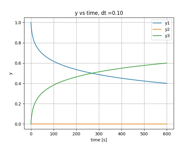
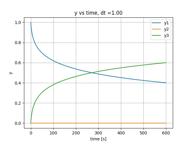
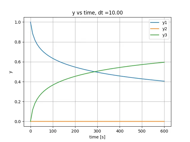
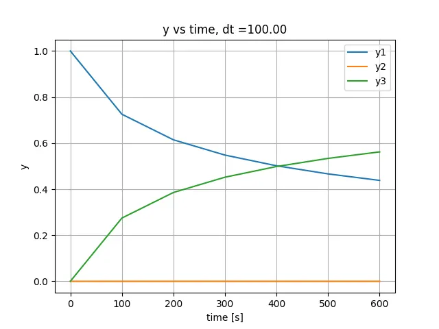
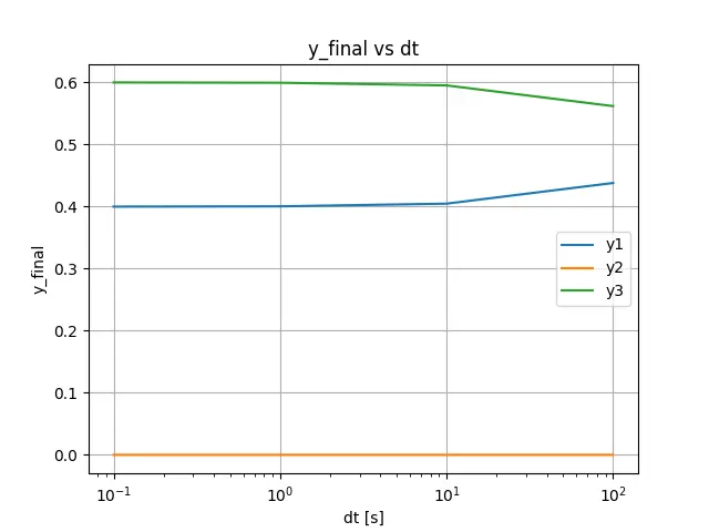
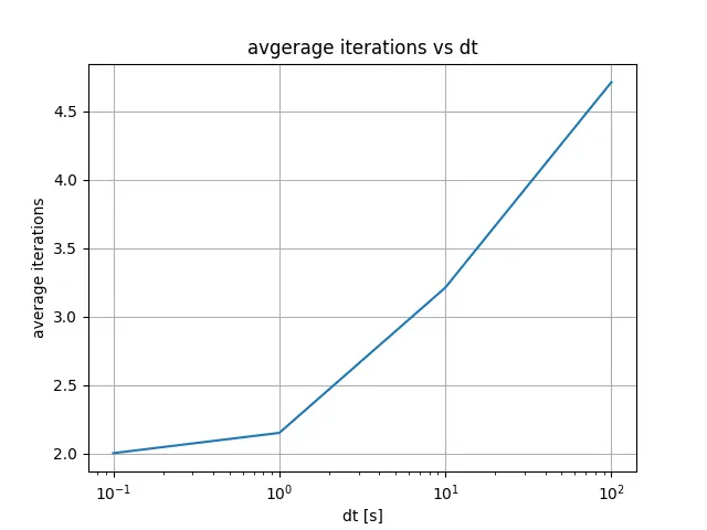
A suitable time-step size depends on the characteristic time-scale of the program and it depends on the simulation objective. Usually time-steps sizes are chosen to be relatively small to avoid sudden changes in values of the flow parameters and reduce the error. Even though backward Euler scheme is unconditionally stable, taking a very large time-step size would lead to sudden changes in parameters and the final result might not be correct. For example, the option of 100 [s] for dt in the plot shows sharp variation in the y curves which must be avoided. Also, as shown in the y final plot, the results for y values are also different for this dt option. For the dt options of 0.1, 1 and 10 [s], the variation of y with time is smooth and all these converge to same results at the end of 10 mins. However with decrease in time-step size, the number of iterations for Newton-Raphson scheme increases as shown in the final plot. So, there is a trade off between the number of iterations and number of time-steps. It is often recommended to have time-step size small enough to have the solutions converge within few iterations for each time-step. This would guarantee converged solution for each time-step and manageable computational cost. Reducing the time-step size too small such as with dt = 0.1 would lead to 6000 time-steps which would lead to large computational time even with less number of iterations. So a choice of dt such as 10 [s] is optimum in this condition since it provides the same result as with dt = 1 [s] and produces a smooth variation of y. In cases, where the problem characteristic time-scales are unknown such as this, a few short simulations with different time-step values can be performed to choose a suitable time-step value such as done above.