Week 6 - Multivariate Newton Rhapson Solver

AIM: Solving the below set of non-linear equations by using multivariate Newton-Raphson solver.

`dy_1/dt=-0.04y_1+10^4*y_2*y_3`........................................(1)

`dy_2/dt=0.04y_1-10^4y_2*y_3-3*10^7*y_2^2`....................(2`

`dy_3/dt=3*10^7*y_2^2`...........................................................(3)

By writing the above equation in backward differencing we get:

`(y_1^n-y_1^(n-1))/(delt)=-0.04y_1^n+10^(4)*y_2^n*y_3^n`....................(4)

`(y_2^n-y_2^(n-1))/(delt)=0.04*y_1^n-10^4*y_2^n*y_3^n-3*10^7*(y_2^2)^n`.................(5)

`(y_3^n-y_3^(n-1))/(delt)=3*10^7*(y_2^2)^n`..................(6)

further simplifying we get:

`y_1^(n-1)+delt(-0.04*y_1^n+10^4*y_2^n*y_3^n)-y_1^n` .................(7)

`y_2^(n-1)+delt(0.04*y_1-10^4*y_2*y_3-3*10^7*y_2^2)-y_2^n` ...............(8)

`y_3^(n-1)+delt(3*10^7*y_2^2)-y_3^n=0` .................................................(9)

let matrix F=`[[f_1],[f_2],[f_3]]`

so when n=1,

`f_1=y_1^0-delt(-0.04*y_1+10^4*y_2*y_3)^1-y_1^(1)=0` .....................(10)

`f_2=y_2^0+delt(0.04*y_1-10^4*y_2*y_3-3*10^7*y_2^2)^1-y_2^1=0` ...............(11)

`f_3=y_3^0+delt(3*10^7*y_2^2)^1-y_3^1=0` ......................................................(12)

so now, `Y_(nw)=Y_(guess)-alpha*J^(-1)F`

import numpy as np 
from numpy.linalg import inv
import matplotlib.pyplot as plt 

# Initial timing
t_init = 0 
# Total time
total_time = 10 # minutes
t_final = total_time*60 #seconds
dt = 0.1
# Number of nodes
n = int((t_final - t_init)/dt)
# Relaxation factor
alpha = 1

# Functions to solve equations

# For 1st equation
def f1(y1,y2,y3,dt,y1_old):
	return (y1_old + dt*(-0.04*y1 + y2*y3*pow(10,4)) - y1) 

# For 2nd equation
def f2(y1,y2,y3,dt,y2_old):
	return (y2_old + dt*(0.04*y1 - y2*y3*pow(10,4) - 3*pow(10,7)*pow(y2,2)) - y2)

# For 3rd equation
def f3(y1,y2,y3,dt,y3_old):
	return (y3_old + dt*(3*pow(10,7)*pow(y2,2)) - y3)


# Function to find Jacobian matrix for provided equations
def jacobi(y1,y1_old,y2,y2_old,y3,y3_old,dt):

	h = 1e-6

	# Jacobian matrix
	j = np.ones((3,3))

	#1st row
	j[0,0] = (f1(y1+h,y2,y3,dt,y1_old) - f1(y1,y2,y3,dt,y1_old))/h
	j[0,1] = (f1(y1,y2+h,y3,dt,y1_old) - f1(y1,y2,y3,dt,y1_old))/h
	j[0,2] = (f1(y1,y2,y3+h,dt,y1_old) - f1(y1,y2,y3,dt,y1_old))/h

	#2nd row
	j[1,0] = (f2(y1+h,y2,y3,dt,y2_old) - f2(y1,y2,y3,dt,y2_old))/h
	j[1,1] = (f2(y1,y2+h,y3,dt,y2_old) - f2(y1,y2,y3,dt,y2_old))/h
	j[1,2] = (f2(y1,y2,y3+h,dt,y2_old) - f2(y1,y2,y3,dt,y2_old))/h

	#3rd row
	j[2,0] = (f3(y1+h,y2,y3,dt,y3_old) - f3(y1,y2,y3,dt,y3_old))/h
	j[2,1] = (f3(y1,y2+h,y3,dt,y3_old) - f3(y1,y2,y3,dt,y3_old))/h
	j[2,2] = (f3(y1,y2,y3+h,dt,y3_old) - f3(y1,y2,y3,dt,y3_old))/h

	return j

# Initial condition at t_init
y1_old = 1 
y2_old = 0
y3_old = 0

y_old = np.ones((3,1))
y_old[0] = y1_old
y_old[1] = y2_old
y_old[2] = y3_old

F = np.copy(y_old)

# Tolerence
tol = 1e-6

Total_iter = 0

# Empty arrays creation
y_1 = []
y_2 = []
y_3 = []
it_mt = []

# Time loop
for i in range(0,n):

	iter = 1
	error = 9e9

	# Space loop
	while tol < error:

		# Calling Jacobi function
		j = jacobi(y_old[0],y1_old,y_old[1],y2_old,y_old[2],y3_old,dt)

		F[0] = f1(y_old[0],y_old[1],y_old[2],dt,y1_old)
		F[1] = f2(y_old[0],y_old[1],y_old[2],dt,y2_old)
		F[2] = f3(y_old[0],y_old[1],y_old[2],dt,y3_old)

		# Finit new guess values for y
		y_new = y_old - alpha*np.matmul(inv(j), F)

		# Calculating error
		error = np.max(np.abs(y_new - y_old))

		# Updating old values (Previous guess values)
		y_old = y_new
		
		# Updating iteration value
		iter = iter + 1

	# End of space loop

	# Printing of matrix after getting coverged values for Y
	log_msg = 'Itereation = {0} y1 = {1} y2 = {2} y3 = {3}'.format(iter, y1_old, y2_old, y3_old)
	print(log_msg)

	# Calculate total number of iterations
	Total_iter = Total_iter + iter

	# Updating old values (Previous time step values)
	y_old = y_new
	y1_old = y_new[0]
	y2_old = y_new[1]
	y3_old = y_new[2]

	y_1.append(y_new[0])
	y_2.append(y_new[1])
	y_3.append(y_new[2])
	it_mt.append(iter)

# End of time loop

# Printing total numbers of iteration
print('Total number of iterations are =',Total_iter)

# Plotting
plt.plot(y_1)
plt.plot(y_2)
plt.plot(y_3)
plt.xlabel('Number of Nodes')
plt.ylabel('Variables')
plt.grid ('on')
plt.legend(['y_1', 'y_2', 'y_3'])
plt.title('For dt = '+str(dt)+'  with number of '+str(Total_iter)+' iterations ')
plt.show()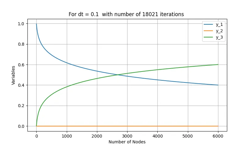

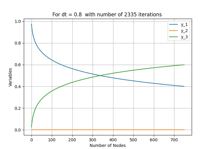
• As the time step dt increases ,the number of iterations decreases the solution converges faster but if we take dt as low value ,we are facing more iterations to converge to the solutions.
• The more accurate results we are getting for lower dt value as the number if grid points increases simultaneously.