Week 6 - Multivariate Newton Rhapson Solver

Objective: To solve the following coupled ordinary differential equation using python programming by Newton Raphson Method.

`(dy_1)/(dt)=-0.04*y_1 + (10^4)*y_2*y_3`

`dy_2/dt=0.04*y_1 - (10^4)*y_2*y_3 -3*(10^7)*y_2^2`

`(dy_3)/(dt)=3*(10^7)*(y_2)^2`

Introduction: In any chemical reaction there are many species are involved the concentration of each species is described by the differential equation, but for reaction concentration of one species is dependent on the concentration of the other species so the system of equation is the coupled differential equation of the concentration of the species. Now for solving the differential equation we will use the implicit method. The formula for the implicit method

`(y_"new"-y_"old")/dt=-0.04*y_1 + (10^4)*y_2*y_3`

`(y_"new"-y_"old")=(-0.04*y_1 + (10^4)*y_2*y_3)*dt`

`f1=(y_"1"-y_"1old")-(-0.04*y_1 + (10^4)*y_2*y_3)*dt=0`

similarly

`f2=y_"2"-y_"2old"-(0.04*y_1 - (10^4)*y_2*y_3 -3*(10^7)*(y_2)^2)*dt=0`

`f3=y_3-y_"3old"-(3*(10^7)*(y_2)^2)*(dt)=0`

`[Y_"new"]=[Y_"old"]-(alpha)*[(J)^(-1)*F]`

Here the Y_new =new values(calculated values)

Y_old=old values(values at previous time step)

J=jacobian matrix

=`[[(df_"1")/(dy_1),(df_"1")/(dy_2),(df_"1")/(dy_3)],[(df_"2")/(dy_1),(df_"2")/(dy_2),(df_"2")/(dy_3)],[(df_"3")/(dy_1),(df_"3")/(dy_2),(df_"3")/(dy_3)]]`

The value for the derivative are calculated numerically

`(df)/(dy)=[f(y+dy)-f(y)]/dy`

F=function vector for y1,y2,y3 values

PYTHON CODE

# solving the coupled differential equation by newton rapshon multivariate method
"""
the differential equation are
          dy1_dt= -0.04*y1 + (10**4)*y2*y3
          dy2_dt=0.04*y1 - (10**4)*y2*y3 -3*(10**7)*y2**2
          dy3_dt =3*(10**7)*y2^2
"""
from ast import Num
from operator import inv

import matplotlib.pyplot as plt
import numpy as np
from numpy.linalg import inv

# defining the function as a name f1,f2,f3 which will return algebric equation by taking inputs y1,y2,y3,y_old,h

def f1(y1,y2,y3,y1_old,h):
    return y1-y1_old-(-0.04*y1 + (10**4)*y2*y3)*h 

def f2(y1,y2,y3,y2_old,h):
    return  y2-y2_old-(0.04*y1 - (10**4)*y2*y3 -3*(10**7)*y2**2)*h

def f3(y1,y2,y3,y3_old,h):
    return y3-y3_old-(3*(10**7)*y2**2)*h
    
# creating the function with name jacobian which will return jacobian(j) of the equation

def jacobian(y1,y2,y3,y_old,h):
    j=np.ones((3,3))
    
    dy=1e-9 # defining the dy to calculate the differentiation of the function f1,f2,f3
    # defining the values of y1_old,y2_old,y3_old which are taken from y_old vector one by one
    y1_old=y_old[0]
    y2_old=y_old[1]
    y3_old=y_old[2]

    # defining the first raw of jacobian
    j[0,0]=(f1(y1+dy,y2,y3,y1_old,h)-f1(y1,y2,y3,y1_old,h))/dy
    j[0,1]=(f1(y1,y2+dy,y3,y1_old,h)-f1(y1,y2,y3,y1_old,h))/dy 
    j[0,2]=(f1(y1,y2,y3+dy,y1_old,h)-f1(y1,y2,y3,y1_old,h))/dy
    # defining the second raw of jacobian
    j[1,0]=(f2(y1+dy,y2,y3,y2_old,h)-f2(y1,y2,y3,y2_old,h))/dy
    j[1,1]=(f2(y1,y2+dy,y3,y2_old,h)-f2(y1,y2,y3,y2_old,h))/dy 
    j[1,2]=(f2(y1,y2,y3+dy,y2_old,h)-f2(y1,y2,y3,y2_old,h))/dy 
     # defining the third raw jacobian
    j[2,0]=(f3(y1+dy,y2,y3,y3_old,h)-f3(y1,y2,y3,y3_old,h))/dy
    j[2,1]=(f3(y1,y2+dy,y3,y3_old,h)-f3(y1,y2,y3,y3_old,h))/dy 
    j[2,2]=(f3(y1,y2,y3+dy,y3_old,h)-f3(y1,y2,y3,y3_old,h))/dy
    
    return j

# defining the time span of 10 minutes of integration at 2000 discrete points
t=np.linspace(0,600,1500)
#to store the y1,y2,y3 at the end of the time iteration
y1=[]
y2=[]
y3=[]    
# defining the time step size 
h=dt=0.01
# defining the initial error to enter into the while loop
error=9e9

#defining the tolerence to control the while loop
tol=1e-6
alpha=1

# defining the y_old vector for initial value  
y_old=np.zeros((3,1))
y_old[0]=1
y_old[1]=0
y_old[2]=0
y_new=np.copy(y_old)
    
# defining the F vector to update it at each iteration
F=np.zeros((3,1))
itr=1
error_itr=np.zeros((200,1))

############################FOR BETTER UNDERSTING OF LOOPS ##################################################

for i in t:
    # extracting the values of y1_old,y2_old andy3_old from y_old vector
    y1_old=y_old[0]
    y2_old=y_old[1]
    y3_old=y_old[2]
    # defining the guess vector
    y_guess=np.copy(y_old)
    ct=1
    # entering the while loop
    while(error>tol):
        # defining the jacobian for time steps
        j=jacobian(y_new[0],y_new[1],y_new[2],y_old,h)

        y1g=y_guess[0]    
        y2g=y_guess[1]
        y3g=y_guess[2]

        # calculating the F vector
        F[0]=f1(y1g,y2g,y3g,y1_old,h)
        F[1]=f2(y1g,y2g,y3g,y2_old,h)
        F[2]=f3(y1g,y2g,y3g,y3_old,h)

        

        # calculating new guess value for next iteration
        y_new=y_guess -alpha*np.matmul(inv(j),F)
        error=max(abs(y_guess-y_new))
        y_guess=y_new
        ct=ct+1
        print(ct)
    
    
    y_old=y_new
    y1.append(y_new[0])
    y2.append(y_new[1])
    y3.append(y_new[2]) 
    error=1e9
    itr=itr+1
    print(itr)

plt.plot(t,y1,color='red',label=r'$y_1$= $\int \frac{dy_{1}}{dt}\,dt$=$\int -0.04y_1 + (10^4)y_2y_3\,dt$')
plt.plot(t,y2,color='green',label=r'$y_2$= $\int \frac{dy_{2}}{dt}\,dt$=$\int 0.04y1 - (10^4)y2y3 -3(10^7)(y2)^2\,dt$')
plt.plot(t,y3,color='black',label=r'$y_3$= $\int \frac{dy_{3}}{dt}\,dt$=$\int 3(10^7)(y2)^2\,dt$')
plt.legend(fontsize=12)
plt.xlabel("t",fontsize=15)
plt.ylabel("y",fontsize=15)
plt.title("Time step size is %f sec " %h)
plt.grid()
plt.show()

OUTPUT

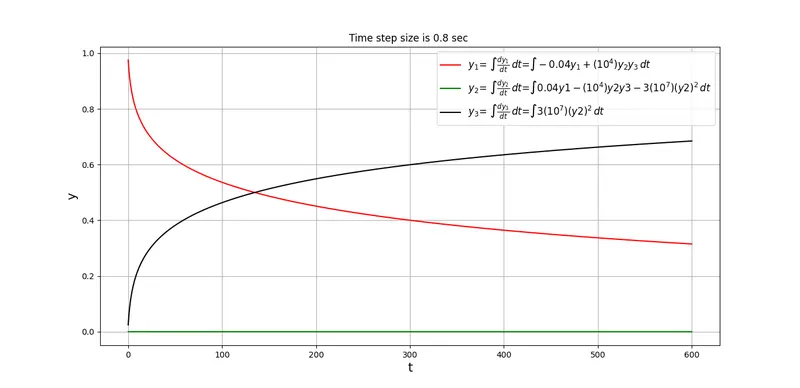
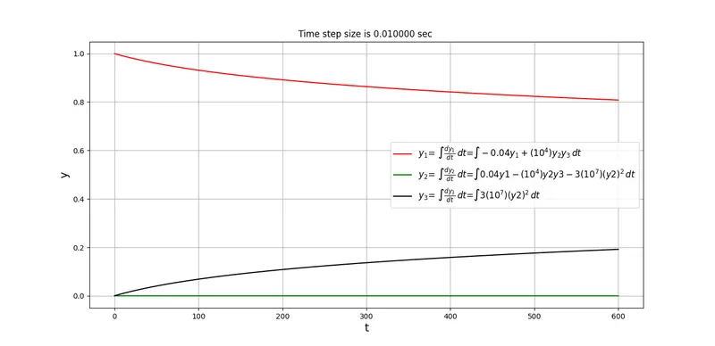
Conclusion:

from the plot at various time steps we can conclude that the phenomena we want to observe are going away with decreasing time step size it is taking more time to evolve fully for the small-time steps so it is required to select the time step size by trial and error method to observe or to examine the particular phenomenon, in this case, it is close to the 0.6 sec because between 0.2 to 0.8 the solution is not changing rapidly.