Week 6 - Multivariate Newton Rhapson Solver

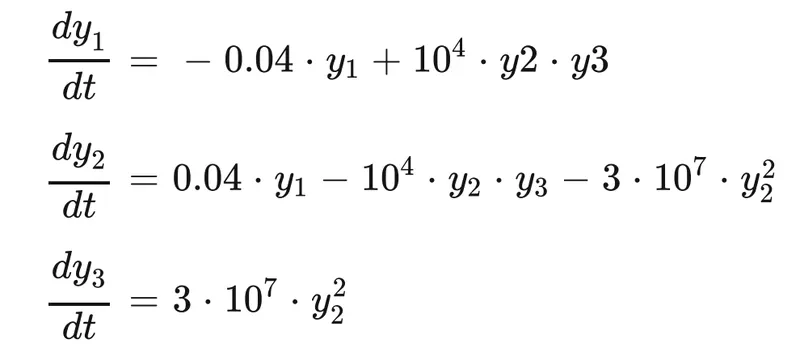
In this challenge, you will solve the set of equations given below,

• f(x) = 0
• f1(x1, x2, x3.... . , xn−1, xn)=0
• f2(x1, x2, x3.... . , xn−1, xn)=0
• f3(x1, x2, x3.... . , xn−1, xn)=0
• .
• .
• .
• fn−1(x1, x2, x3.... . , xn−1, xn)= 0
• fn(x1, x2, x3.... . , xn−1, xn) = 0

We will adopt the compact form notation for the equation:

F(X_i)=0==> Contains functions with i numbers of variables to be solved for

According to Multi-variate Newton Raphson Method,

Where F is a vector of the functions given in the function and the size of (no_variables, 1)

Y_new and Y_old are vecotors used to store the values of the variables of interest. The size is also (no_variables ,1)

alpha is the relaxation factor

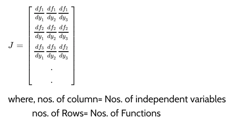
J is the Jacobian matrix

The Python code is as follows:

"""
This code is written by Mr. Noble Sahrma as a part of the TSE CFD training
Used to solve the system of differntial equations using Newton Rhapsons method
"""
import numpy as np
import matplotlib.pyplot as plt
from numpy.linalg import inv

# Functions to solve each multivariable equation
def F1(y,y_old1,h): 

	Function1= y_old1 + h*(-0.04*y[0] + (pow(10,4)*y[1]*y[2])) - y[0]
	return Function1

def F2(y,y_old2,h): 
	Function2= y_old2 + h*(0.04*y[0] - (pow(10,4)*y[1]*y[2]) - (3*pow(10,7)*pow(y[1],2))) - y[1]
	return Function2

def F3(y,y_old3,h): 
	
	Function3= y_old3 + h*(3*pow(10,7)*pow(y[1],2)) - y[2]
	return Function3

## Defining the jacobi function to evalaute the jacobi ##############
def jacobian(y_new,y_old,h):
	# input an identity 3x3 matrix
	Jacobi = np.ones((3,3))
	# Using dummy values that will be updated for each time step when solving
	# To solve the system numerically
	dy = 1e-10

	Y1=[y_new[0]+dy,y_new[1],y_new[2]]
	Y2=[y_new[0],y_new[1]+dy,y_new[2]]
	Y3=[y_new[0],y_new[1],y_new[2]+dy] 


	Jacobi[0,0] = (F1(Y1,y_old[0],h) - F1(y_new,y_old[0],h))/dy
	Jacobi[0,1] = (F1(Y2,y_old[1],h) - F1(y_new,y_old[1],h))/dy
	Jacobi[0,2] = (F1(Y3,y_old[2],h) - F1(y_new,y_old[2],h))/dy
	
	Jacobi[1,0] = (F2(Y1,y_old[0],h) - F2(y_new,y_old[0],h))/dy
	Jacobi[1,1] = (F2(Y2,y_old[1],h) - F2(y_new,y_old[1],h))/dy
	Jacobi[1,2] = (F2(Y3,y_old[2],h) - F2(y_new,y_old[2],h))/dy
	
	Jacobi[2,0] = (F3(Y1,y_old[0],h) - F3(y_new,y_old[0],h))/dy
	Jacobi[2,1] = (F3(Y2,y_old[1],h) - F3(y_new,y_old[1],h))/dy
	Jacobi[2,2] = (F3(Y3,y_old[2],h) - F3(y_new,y_old[2],h))/dy
	return Jacobi

##### The Main program begins here ####

# Input the guess values as old, due to use of backward differencing
y_old = np.zeros((3,1))
y_old[0] = 1
F = np.zeros((3,1))  # Function value 

y_new = np.zeros((3,1)) # Array to store the values for the iteration in the rhapson methd
# inputs
alpha = 1 # alpha for Newton raphson solver
tol = 1e-10  # tolereance
error = 1e9  # error variable to terminate the process
h=0.1 # Time stamp
Time_Simulation=np.arange(0,600, h) # creating an array of time for simulation 

# Empty arrays initialized for storing final values
e = np.zeros((int(600/h),1)) # Used to store the error 

Y1 = np.zeros((3, int(600/h))) # Used to stor ethe values of Y1 Y2 Y3 along the time steps

for i in range (0, len(Time_Simulation)):
	
	y_guess = np.copy(y_old)
	while error > tol:
		# computing jacobian - old values used
		J = jacobian(y_new,y_old,h)
		# Computing F vector - old values used
		F[0] = F1(y_guess, y_old[0],h)
		F[1] = F2(y_guess, y_old[1],h)
		F[2] = F3(y_guess, y_old[2],h)
		# computing new values
		y_new = y_guess - alpha*np.matmul(inv(J),F)
		error = max(abs(y_new-y_guess))
		y_guess = y_new
	# Values after each time step added into array
	e[i] = error
	y_old = y_new
	Y1[:, i] = y_new[:,0]
	error = 1e9

# Plots
plt.plot(Time_Simulation,Y1[0, :], label = 'y1')
plt.plot(Time_Simulation,Y1[1,:], label = 'y2')
plt.plot(Time_Simulation,Y1[2, :], label = 'y3')
plt.title('Multi-variate Newton Raphson Solver for dt = ' +str(h))
plt.xlabel('Time (secs)')
plt.ylabel('$y_i$')
plt.legend()
plt.grid()
plt.show()

Code written is compact and needs minute corrections to vary the alpha and other parameters

the Output curve:

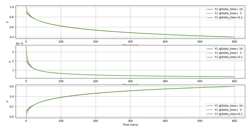
For the time step dt, we must assume the best value that gives a fairly accurate result for the problem. If we take dt as 1, there are 600 steps in the system and hence results are sharp and not that accurate.

The delta time is taken as 10, 5 and 0.1. It can be seen tha the error is lower in case of lower delat (time). The convergence is almost the same in all thre three cases