Week 6 - Multivariate Newton Rhapson Solver

MULTIVARIANT NEWTON RAPHSON METHOD FOR SOLVING STIFF ODE's

Objective:

• To Solve the problem using Implicit Euler Method/Backward Differencing, assume the initial conditions as y1 = 1, y2 = 0, and y3 = 0 respectively. Also take alpha (relaxation factor) = 1 and Simulation time t = 10 minutes.
• Choose a suitable step size and explain the reason for choosing that step size and also mention what is the ideal step size in this case?

Given Problem:

The set of equations to be solved are :-

`(dy1)/dt = -0.04*y1 + 10^4*y2*y3`

`(dy2)/dt = 0.04*y1-10^4y2*y3-3.10^7*y2^2`

`(dy3)/dt = 3.10^7*y2^2`

As we see It is a coupled non-linear equation which has to be solved. To solve this equations we are going to use Multivariant Newton's Raphson Method to find the roots. Newton Raphson's method is a iterative technique which is used to solve the roots of an non-linear equations. These equations are designed as reaction ODE's and that's why it is going to Stiff ODE's and We solve this ODE's by Implicit Backward Differencing Method.

Ynew = Yold - α*inv(J)*F

here,

Y new = New values for Y after each iteration

Yold = Initial guess values for Y to start the iteration

Alpha(α) = Relaxation factor

inv(J) = Inverse of Jacobian Matrix which gives us the all possible derivatives for each variable in each function.

F = Function Matrix

As per the Challenge given, Jacobian matrix has to find numerically which is defined as below:

`Y^(n ew)` = `[[Y^(n ew)],[Y^(n ew)],[Y^( n ew)]]`

`Y^(o l d)= [[Y^(o l d)],[Y^(o l d)],[Y^( ol d)]]`

`J` = `[[(df1)/(dy1),(df1)/(dy2),(df1)/(dy3)],[(df2)/(dy1),(df2)/(dy2),(df2)/(dy3)],[(df3)/(dy1),(df3)/(dy2),(df3)/(dy3)]]`

To convert the above differential equations into non-linear equations, we are using backward differencing Scheme called Implicit Euler Method:

`f'(x i)` = `(f(x i) - f(x i-1))/dx`

`(dy)/dx = f(yi)`

`(yi^n - yi^(n-1))/dt = f(yi)`

`yi^(n-1) + f(yi) *dt - y^n = 0`

The above set of equations at time step n =1,

`f1 = y1^0 + (-0.04*y1 + 10^4*y2*y3) *(dt) - y1^1`

`f2 = y2^0 + (0.04*y1 + 10^4*y2*y3 - 3.10^7*y2^2) *(dt) - y2^1`

`f3 = y3^0 + (3.10^7*y2^2) *(dt) - y3^1`

Similarly, we will iterate the system for 10 mins with various given time steps to find the roots of the equations. The initail guesses for the y values are also given in the baove challenge as y1 = 1, y2= 0, y3 = 0.

Python code:-

"""
Program on Multivaraiant Newphton Raphson method to solve Non-linear coupled equations

dY1/dt = -0.04*y1 + 10^4*y2*y3 y
dY2/dt = 0.04*y1 -10^4*y2*y3 - 3.10^7*y2^2
dY3/dt = 3.10^7*y2*2
"""
import numpy as np 
import matplotlib.pyplot as plt 
from numpy.linalg import inv

#Defining the functions
def f1(y1_old, y1, y2, y3,dt):
	return (y1_old + dt*(-0.04*y1 + 1e4*y2*y3) -y1)

def f2(y2_old, y1, y2, y3,dt):
	#return (y2_old + dt*((-0.04*y1) + (1e4*y2*y3)- (3e7*y2*y2)) -y2)
	return (y2_old + dt*((0.04*y1) - (1e4*y2*y3)- (3e7*y2*y2)) -y2)

def f3(y3_old, y1, y2, y3,dt):
	#return (y1_old + dt*(3e7*y2*y2)-y3)
	return (y3_old + dt*(3e7*y2*y2)-y3)

#Defining the jacobian matrix which gives us possible derivate for each term
def jacobian(y1_old, y2_old, y3_old, y1, y2, y3, dt):
	"""
	creating the Jacobian 3*3 Matrix  
	"""
	J = np.ones((3,3))
	"""
	Step size
	"""
	dy = 1e-6

	#Row1
	J[0,0] = (f1(y1_old,y1+dy,y2,y3,dt)-f1(y1_old,y1,y2,y3,dt))/dy
	J[0,1] = (f1(y1_old,y1,y2+dy,y3,dt)-f1(y1_old,y1,y2,y3,dt))/dy
	J[0,2] = (f1(y1_old,y1,y2,y3+dy,dt)-f1(y1_old,y1,y2,y3,dt))/dy

	#Row2
	#J[1,0] = (f2(y1_old,y1+dy,y2,y3,dt)-f2(y1_old,y1,y2,y3,dt))/dy
	J[1,0] = (f2(y2_old,y1+dy,y2,y3,dt)-f2(y2_old,y1,y2,y3,dt))/dy
	#J[1,1] = (f2(y1_old,y1,y2+dy,y3,dt)-f2(y1_old,y1,y2,y3,dt))/dy
	J[1,1] = (f2(y2_old,y1,y2+dy,y3,dt)-f2(y2_old,y1,y2,y3,dt))/dy
	#J[1,2] = (f2(y1_old,y1,y2,y3+dy,dt)-f2(y1_old,y1,y2,y3,dt))/dy
	J[1,2] = (f2(y2_old,y1,y2,y3+dy,dt)-f2(y2_old,y1,y2,y3,dt))/dy

	#Row3
	#J[2,0] = (f3(y1_old,y1+dy,y2,y3,dt)-f3(y1_old,y1,y2,y3,dt))/dy
	J[2,0] = (f3(y3_old,y1+dy,y2,y3,dt)-f3(y3_old,y1,y2,y3,dt))/dy
	#J[2,1] = (f3(y1_old,y1,y2+dy,y3,dt)-f3(y1_old,y1,y2,y3,dt))/dy
	J[2,1] = (f3(y3_old,y1,y2+dy,y3,dt)-f3(y3_old,y1,y2,y3,dt))/dy
	#J[2,2] = (f3(y3_old,y1,y2,y3+dy,dt)-f3(y1_old,y1,y2,y3,dt))/dy
	J[2,2] = (f3(y3_old,y1,y2,y3+dy,dt)-f3(y3_old,y1,y2,y3,dt))/dy
	return J

#Defining the initial guess values for variables
y1_old = 1
y2_old = 0
y3_old = 0


#numpy column Vector 
Y_old = np.ones((3,1))
Y_old[0] = y1_old
Y_old[1] = y2_old
Y_old[2] = y3_old

#numpy column vector F
F = np.copy(Y_old)

#parameters for newton raphson solver
aplha = 1

t = 600 #simulation time 
dt = 10 #time step
n = int(t/dt) #number of time steps

#creating solver paramter
y1= []
y2 = []
y3 = []
iteration = []

iter = 1
for i in range(0,n):
	error = 9e9
	tol = 9e-6
	
	while error >tol:
		#computing the jacobian - old values are used

		J = jacobian(y1_old, y2_old, y3_old, Y_old[0], Y_old[1], Y_old[2], dt);

		F[0] = f1(y1_old, Y_old[0], Y_old[1], Y_old[2],dt);
		F[1] = f2(y2_old, Y_old[0], Y_old[1], Y_old[2],dt);
		F[2] = f3(y3_old, Y_old[0], Y_old[1], Y_old[2],dt);

		#computing new values 
		Y_new = Y_old-aplha*np.matmul(inv(J),F)

		#computing max abs error 
		error = np.max(np.abs(Y_new - Y_old))

		#updating the old values
		Y_old = Y_new 
		#log message 
		log_message = 'iteration = {0} y1 = {1} y2 = {2} y3 = {3}'.format(iter, Y_new[0],Y_new[1],Y_new[2])
		print(log_message)
		iter = iter+1
	
	y1.append(Y_new[0])
	y2.append(Y_new[1])
	y3.append(Y_new[2])
	iteration.append(iter)

	#final results 
	Y_old = Y_new
	y1_old = Y_new[0] 
	y2_old = Y_new[1] 
	y3_old = Y_new[2]	

		
plt.plot(iteration,y1)
plt.plot(iteration,y2)
plt.plot(iteration,y3)
plt.xlabel('time:' + str(dt*n))
plt.ylabel('variables')
plt.title('Multivaraiant Newton Raphson Method for :' +str(dt))
plt.legend(['y1','y2','y3'])
plt.grid('on')
plt.show()

Coding Approach:-

• First of all we have to write the given equations and convert them into Root finding equations.
• Import all the essential Libararies to do the simulation.
• Defining the Functions as in the form of given equations with the desired Inputs.
• Then defining the Jacobian matrix and solving the function numerically by each variable.
• Defining the Initial guess values for y.
• After that we have create the Y_old matrix and using the initial guess values as a function.
• Defining all the time related data as simulation time as 600 secs with situable time step size.
• After that We start the Newton Raphson method outer time loop by assembling the ODE system inside a while loop.
• Then run the While loop with conditions as errror>tol It converges till this given Condition and updating the y_old values for next iterations at each Iteration.
• We Obtained the new values by using append the values and then plot the results.

Results:-

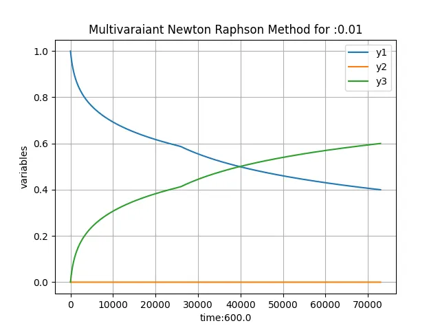
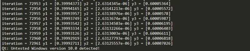
For dt = 0.01

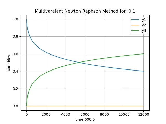
For dt = 0.1

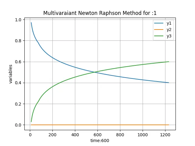
dt = 1

dt = 10

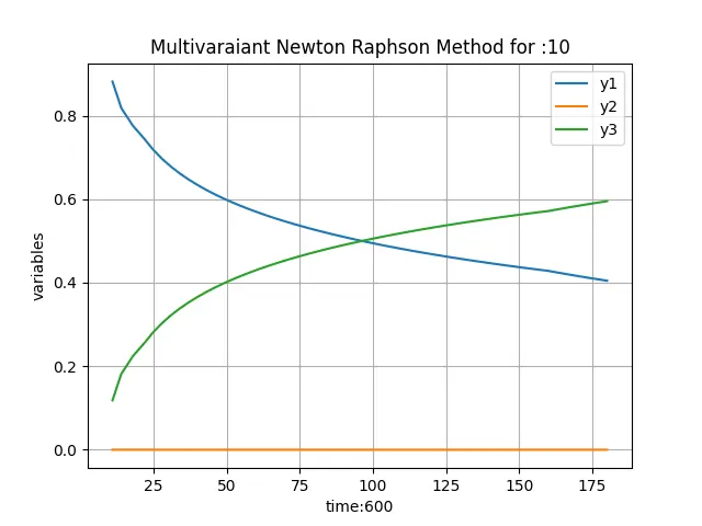
As you see we got mostly similar plots But for the Accuracy of the plots we increase the number of Time Step size from 0.01 to 10 ms. By increasing the time step the number of iterations is also we got less as compared time step size 0.01 ms. It means we get convergence solution as we increase the Time Step and Also it takes very less time as compared for the step size 0.01. If we further decrease the Time Step size It takes more time to get the convergence solution It is Because It have to Solve for more iterations. By keeping simulation time and Accuracy in mind, the time step of 0.1s is situable for this Challenge.