Week 6 - Multivariate Newton Rhapson Solver
Multivariate Newton Rhapson Solver
Aim:
To solve set of coupled ordinary differential equations using Implicit Euler Method/Backward Differencing for discretizing, multivariate Newton Rhapson Method for solving the non-linear algebraic equations obtained from discretization and numerical differentiation for calculating the Jacobian matrix.
Given Informattion:
The following information is given regarding the problem:
Differential equations to be solved are
`(dy_1)/(dt) = -0.04y_1 + 10^4y_2y_3`
`(dy_2)/(dt) = 0.04y_1 - 10^4y_2y_3 - 3*10^7y_2^2`
`(dy_3)/(dt) = 3*10^7y_2^2`
Initial consitions are
`y_1 = 1,y_2 = 0 and y_3 = 0`
Relaxation factor in Newton Rhapson method is alpha = 1.
Simulation run time is 10 minutes.
Procedure Followed:
By preforming discretization, using implicit Euler Method/ Back-ward differencing.
`y_1^n = y_1^(n-1) + h*( -0.04y_1^n + 10^4y_2^ny_3^n)`
`y_2^n=y_2^(n-1)+h*(0.04y_1^n - 10^4y_2^ny_3^n - 3*10^7(y_2^n)^2)`
`y_3^n = y_3^(n-1) + h*(3*10^7(y_2^n)^2)`
where 'h' is the time step for numerical integration.
We get non-linear algebraic equation which are to be solved at each and every time step using Multivariate Newton-Rhapson Method.
Rearranging above equations, we get
`y_1^(n-1) + h*( -0.04y_1^n + 10^4y_2^ny_3^n) -y_1^n = 0`
`y_2^(n-1)+h*(0.04y_1^n - 10^4y_2^ny_3^n - 3*10^7(y_2^n)^2) - y_2^n = 0`
`y_3^(n-1) + h*(3*10^7(y_2^n)^2) - y_3^n = 0`
These equations can be represented as
`f_1(y_1^n,y_2^n,y_3^n) = 0`
`f_2(y_1^n,y_2^n,y_3^n) = 0`
`f_3(y_1^n,y_2^n,y_3^n) = 0`
We need to solve these equations at each and every time step.
Jacobian Matrix is required to be calculated for Multi-Variate Newton Rhapson Method.
`Jacobian Matrix = J = [[(delf_1)/(dely_1),(delf_1)/(dely_2),(delf_1)/(dely_3)],[(delf_2)/(dely_1),(delf_2)/(dely_2),(delf_2)/(dely_3)],[(delf_3)/(dely_1),(delf_3)/(dely_2),(delf_3)/(dely_3)]]`
The elements of the Jacobian Matric are the partial derivatives of 'f' w.r.t. 'y'.
These derivatives are calculated numerically.
Code:
Code used for solving the differential equations.
"""
python code for solving system of coupled non-linear differential equations

iteration formula  for multi variate newton raphson method is xn+1 = xn - alpha*J^(-1)*F(xn)
`(dy1)/(dt) = -0.04y1 + 10^4y2y3`

`(dy2)/(dt) = 0.04y1 - 10^4y2y3 - 3*10^7y2^2`

`(dy3)/(dt) = 3*10^7y2^2`

f1, f2, f3 obtained after discretization are
`y1^(n-1) + h*( -0.04y1^n + 10^4y2^ny3^n) -y1^n = 0`

`y2^(n-1)+h*(0.04y1^n - 10^4y2^ny3^n - 3*10^7(y2^n)^2) - y2^n = 0`

`y3^(n-1) + h*(3*10^7(y2^n)^2) - y3^n = 0`
Modules required are
1. numpy is required for matrix multiplication
2. inv is required for computing the inverse of a matrix
"""
import numpy as np
from numpy.linalg import inv
import matplotlib.pyplot as plt


def f1(y1n,y2n, y3n,y1m,y2m, y3m,h):
	"""
	first non linear function obtained from BDS of first ODE
	n is previous time step values
	m means present time step values
	"""
	return (y1n + h*(-0.04*y1m + pow(10,4)*y2m*y3m) - y1m)

def f2(y1n,y2n ,y3n,y1m,y2m ,y3m,h):
	"""
	first non linear function obtained from BDS of second ODE
	n is previous time step values
	m means present time step values
	"""
	return (y2n + h*(0.04*y1m - pow(10,4)*y2m*y3m - 3*pow(10,7)*pow(y2m,2)) - y2m)
def f3(y1n,y2n ,y3n,y1m,y2m ,y3m,h):
	"""
	first non linear function obtained from BDS of third ODE
	n is previous time step values
	m means present time step values
	"""
	return (y3n + h*(3*pow(10,7)*pow(y2m,2)) - y3m)
def jacobian(y1n,y2n, y3n,y1m,y2m, y3m,h):
	"""
	defining the jacobian matrix
	"""
	# 3 by 3 unit matrix
	J = np.ones((3,3))
	# small change in y
	dy = 1e-6

	#Row 1
	J[0,0] = (f1(y1n,y2n, y3n,y1m+dy,y2m, y3m,h)-f1(y1n,y2n, y3n,y1m,y2m ,y3m,h))/dy
	J[0,1] = (f1(y1n,y2n, y3n,y1m,y2m+dy, y3m,h)-f1(y1n,y2n, y3n,y1m,y2m ,y3m,h))/dy
	J[0,2] = (f1(y1n,y2n, y3n,y1m,y2m, y3m+dy,h)-f1(y1n,y2n, y3n,y1m,y2m ,y3m,h))/dy

	#Row 2
	J[1,0] = (f2(y1n,y2n, y3n,y1m+dy,y2m, y3m,h)-f2(y1n,y2n, y3n,y1m,y2m, y3m,h))/dy
	J[1,1] = (f2(y1n,y2n, y3n,y1m,y2m+dy, y3m,h)-f2(y1n,y2n, y3n,y1m,y2m ,y3m,h))/dy
	J[1,2] = (f2(y1n,y2n, y3n,y1m,y2m ,y3m+dy,h)-f2(y1n,y2n, y3n,y1m,y2m ,y3m,h))/dy


	#Row 3
	J[2,0] = (f3(y1n,y2n, y3n,y1m+dy,y2m ,y3m,h)-f3(y1n,y2n, y3n,y1m,y2m, y3m,h))/dy
	J[2,1] = (f3(y1n,y2n, y3n,y1m,y2m+dy, y3m,h)-f3(y1n,y2n, y3n,y1m,y2m, y3m,h))/dy
	J[2,2] = (f3(y1n,y2n, y3n,y1m,y2m, y3m+dy,h)-f3(y1n,y2n, y3n,y1m,y2m, y3m,h))/dy

	return J

# defining the initial conditions
y1_initial= 1
y2_initial = 0
y3_initial = 0

# array for storing variables at each time step
y = np.ones((3,1))
y[0] = y1_initial
y[1] = y2_initial
y[2] = y3_initial
plt.plot(0,y[0],'.',color = 'red')
plt.plot(0,y[1],'.',color = 'green')
plt.plot(0,y[2],'.',color = 'blue')
# simulation time in sec
time = 600
# time step size
h = 0.1# sec


# numpy column vector
y_old = np.ones((3,1))

# numpy column vecor for F
F = np.copy(y_old)

# parameters for the newton raphson solver
alpha = 1
tol = 1e-16
# starting integration loop
for i in range (0,6000):
	j = i+1
	# inital error
	error = 9e9
	y_old[0]=y[0]
	y_old[1]=y[1]
	y_old[2]=y[2]

	# starting the newton raphson loop
	#iteration = 0
	while error > tol:

		# computing the Jacobian - old values are used
		J = jacobian(y[0],y[1],y[2],y_old[0],y_old[1],y_old[2],h)
		# computing the F vector - old values are used
		F[0]=f1(y[0],y[1],y[2],y_old[0],y_old[1],y_old[2],h)
		F[1]=f2(y[0],y[1],y[2],y_old[0],y_old[1],y_old[2],h)
		F[2]=f3(y[0],y[1],y[2],y_old[0],y_old[1],y_old[2],h)

		# computing new values
		y_new = y_old - alpha*np.matmul(inv(J),F)

		# computing max abs error
		error = np.max(np.abs(y_new-y_old))

		# updating old values
		y_old = y_new

		#iteration = iteration +1

		# log message
		#log_message = 'iteration number # = {0} 1 = {1} x2 = {2} x13 = {3}'.format(iteraton,y_new[0],y_new[1],y_new[2])
		#print(log_message)
	y[0] = y_new[0]
	y[1] = y_new[1]
	y[2] = y_new[2]
	print('y1 = {0} y2={1} y3 = {2}'.format(y[0],y[1],y[2]))
	if j%1== 0:
		plt.plot(j*h,y[0],'.',color = 'red')
		plt.plot(j*h,y[1],'.',color = 'green')
		plt.plot(j*h,y[2],'.',color = 'blue')


# final results
print('y1 = {0} y2={1} y3 = {2}'.format(y[0],y[1],y[2]))
plt.xlabel("time")
plt.ylabel("y values")
plt.title("Solution of given differential equations")
plt.grid('on')
plt.legend(["y1","y2","y3"])
plt.show()
Plots:
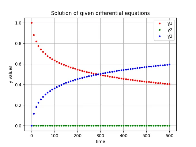
Case-1:
dt = 10, number of time steps = 60

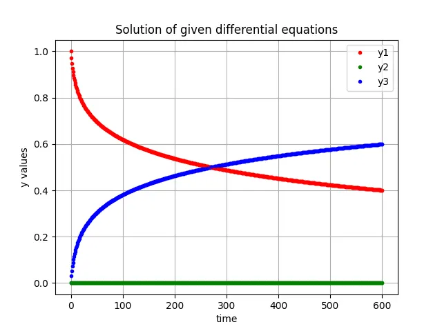
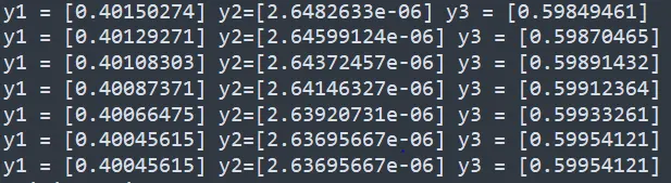
Case-2:
dt = 1, number of time steps = 600
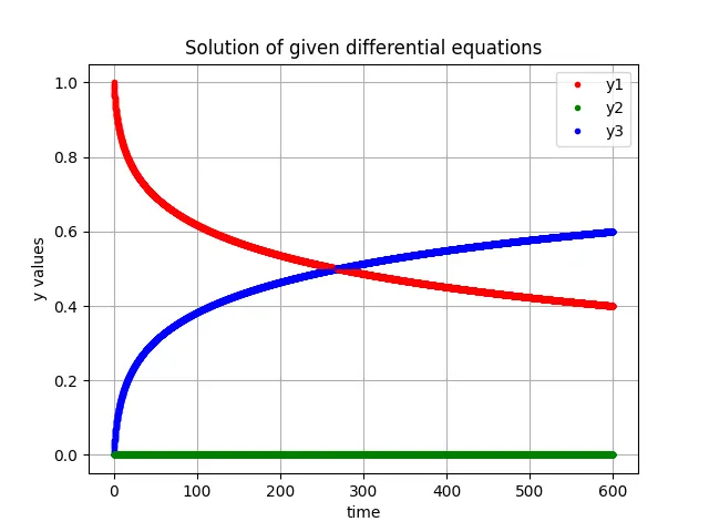
Case-3:
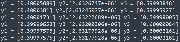
dt = 0.1, number of time steps = 6000
Case-4:
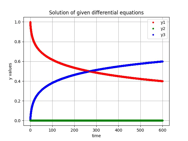
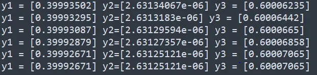
dt = 0.01, number of time steps = 60000
Comments:
From the above results obtained at each time step value, we can see that the values of `y_1`, `y_2` and `y_3` at the end of simulation are varying. So, we can conclude that there is no specific value of time step which is ideal universally. Depending on the accuracy of the solution needed, we choose time step. There is no restriction on time step value from stability point of view as we used Implicit Euler differencing.