Week 6 - Multivariate Newton Rhapson Solver
Multivariate Newton Rhapson Solver
Aim:
writing a code to solve the set of ODE equations with multi variables using Multivariate Newton Rhapson Solver. use Implicit Euler Method/Backward Differencing for jacobian matrix.
Equations:
`dy_1/dt = -0.04*y_1 + 10^4*y_2*y_3 ------------(1)`
`dy_2/dt = 0.04*y_1 - 10^4*y_2*y_3 - 3*10^7*y_2^2 ---------(2)`
`dy_3/dt = 3*10^7*y_2^2 -----------------(3)`
Solution Procedure:-
To solve multivariable system of equations we use Multivariate Newton Rhapson Solver
The Newton-Raphson method is a way to quickly find a good approximation for the root of a real-valued function `f ( x ) = 0`. It uses the idea that a continuous and differentiable function can be approximated by a straight line tangent to it.
for single variable:-
`x_(text(new))=x_(guess)-alpha**[f(x_(guess))/(f'(x_(guess)))]`
`alpha` = relaxation factor
for multivariable problem:-
`x_(text(new))=x_(guess)-alpha**(J^(-1)**F)_(guess)`
where ,
J = Jacobian matrix of the couples equations.
Newton-Raphson method is used with the analytical solution of the Jacobian matrix to give an iterative solution of pole placement equations with better percentage success rate than the other methods quoted in literature.
for this case J is,
`J = [[(df_1)/dy_1,(df_1)/dy_2,(df_1)/dy_3],[(df_2)/dy_1,(df_2)/dy_2,(df_2)/dy_3],[(df_3)/dy_1,(df_3)/dy_2,(df_3)/dy_3]]`
F = Function matrix
matrix formed by system of coupled non linear equations.
`F = [[f_1],[f_2],[f_3]]`
Procedure to obtain function matrix:-
Use Backward differencing scheme to descritise the above equations 1 , 2, 3.
`f^' (x_i )= (f(x_i )-f(x_(i-1)))/(Deltax )`
`Deltax =` Step size
`((y_1^n)-(y_1^(n-1)))/(Deltat) = -0.04(y_1^n)+10^4(y_2^n)(y_3^n)`
`((y_2^n)-(y_2^(n-1)))/(Deltat) = 0.04(y_1^n)-10^4(y_2^n)(y_3^n) - 3*10^7*(y_2^n)^2`
`((y_3^n)-(y_3^(n-1)))/(Deltat) = 3*10^7*(y_2^n)^2`
`Delta t = h = time step`
`y_1^n=y_1^(n-1)+h.(-0.04*y_1^n+10^4*y_2^n*y_3^n)`
`y_2^n=(y_2^(n-1))+h.(0.04(y_1^n)-10^4(y_2^n)(y_3^n)-3**10^7(y_2^2)^n)`
`y_3^n=(y_3^(n-1))+h.(3**10^7(y_2^2)^n)`
To find roots of the we have to equate the equations to 0.
The function form of equations are:-
`f_1=y_1^(n-1)+h.(-0.04*y_1^n+10^4*y_2^n*y_3^n)-y_1^n=0`
`f_2=(y_2^(n-1))+h.(0.04(y_1^n)-10^4(y_2^n)(y_3^n)-3**10^7(y_2^2)^n)-y_2^n=0`
`f_3=(y_3^(n-1))+h.(3**10^7(y_2^2)^n)-y_3^n=0`
`F = [[f_1],[f_2],[f_3]]`
Given Data:-
Initial conditions:
`[[Y_1 = 1],[Y_2 = 0],[Y_3 = 0]]`
`text(Relaxation factor ) => alpha =1`
`text(simulation time)= 10 min =600 sec`
Program Procedure:
- Import the required libraries and modules, like numpy, matplotlib , inv in numpy.
- Define the functions `f_1,f_2,f_3`
- Write function code to calculate Jacobian matrix.
- Give initial values and guess values. take both as same to reduce number of steps.
- Declare the values like `alpha = 1`, `dy = 1e-6`,`text(tolerance) = 1e-12`,`dt = [100,50,25,10,5,2.5,1,0.5,0.1]`
- dy = step size ; dt = h= array of time steps.
- Create a time step loop to analyze solutions for different time step sizes
- Outer time integration loop
- Assembling of ODE system
- Run the Newton Raphson till the solution Converges
- Get New values + Perform required updates
- End time loop
- End Time step loop
- Plot the results.
- Give conclusions.
Main Program:-
'''
Program to solve the system of coupled non-linear equations
	y1_old + h*(-0.04*y1 + pow(10,4)*y2*y3)-y1 = 0
	y2_old + h*(0.04*y1 - pow(10,4)*y2*y3 - 3*pow(10,7)*pow(y2,2))-y2 = 0
	y3_old + h*(3*pow(10,7)*pow(y2,2))-y3 = 0
	h = dt = time step
Modules required
1. numpy is required for matrix multiplication
2. inv is required for computing the inverse of a matrix
3. matplotlib is required to plot the results
'''
import numpy as np
from numpy.linalg import inv
import matplotlib.pyplot as plt

def f1(y1, y2, y3, y1_old, h):
	# First non-linear equation
	return y1_old + h*(-0.04*y1 + pow(10,4)*y2*y3)-y1

def f2(y1, y2, y3, y2_old, h):
	# Second non-linear equation
	return y2_old + h*(0.04*y1 - pow(10,4)*y2*y3 - 3*pow(10,7)*pow(y2,2))-y2

def f3(y1, y2, y3, y3_old, h):
	# third non-linear equation
	return y3_old + h*(3*pow(10,7)*pow(y2,2))-y3

def jacobian(y1, y2, y3, y1_old, y2_old, y3_old, h, dy):
	# Defining the Jacobian
	#3 by 3 unit matrix
	J = np.ones((3,3))

	# Row 1 df(n)/dy(n) = (f(n+1)-f(n))/dy
	J[0,0] = (f1(y1+dy, y2, y3, y1_old, h)-f1(y1, y2, y3, y1_old, h))/dy    # df1/dy1
	J[0,1] = (f1(y1, y2+dy, y3, y1_old, h)-f1(y1, y2, y3, y1_old, h))/dy    # df1/dy2
	J[0,2] = (f1(y1, y2, y3+dy, y1_old, h)-f1(y1, y2, y3, y1_old, h))/dy    # df1/dy3

	# Row 2
	J[1,0] =  (f2(y1+dy, y2, y3, y2_old, h)-f2(y1, y2, y3, y2_old, h))/dy    # df2/dy1
	J[1,1] =  (f2(y1, y2+dy, y3, y2_old, h)-f2(y1, y2, y3, y2_old, h))/dy    # df2/dy2
	J[1,2] =  (f2(y1, y2, y3+dy, y2_old, h)-f2(y1, y2, y3, y2_old, h))/dy    # df2/dy3

	# Row 3
	J[2,0] = (f3(y1+dy, y2, y3, y3_old, h)-f3(y1, y2, y3, y3_old, h))/dy    # df3/dy1
	J[2,1] = (f3(y1, y2+dy, y3, y3_old, h)-f3(y1, y2, y3, y3_old, h))/dy    # df3/dy2
	J[2,2] = (f3(y1, y2, y3+dy, y3_old, h)-f3(y1, y2, y3, y3_old, h))/dy    # df3/dy3

	return J


# parameters for newton rhapson solver
alpha = 1
dy = 1e-6
dt = [100,50,25,10,5,2.5,1,0.5,0.1] # Time step
# dt = [0.1,] # Time step
tol   = 1e-10
fig = 1
for h in dt:
	#numpy column vector for old values (previous time step values)
	Y_old = np.zeros((3,1))
	Y_old[0] = 1

	#numpy column vector initial guess values g = guess
	Y_g = np.copy(Y_old)

	#numpy column vector for F
	F = np.copy(Y_g)

	Y1 = []
	Y2 = []
	Y3 = []
	t = np.arange(0,600,h)  # Time
	print(h)

	# Starting the newton rhapson loop
	for i in range(0,len(t)):
		# print(i)
		error = 9e9
		while error > tol:
			# Computing the Jacobian old values are used
			J = jacobian(Y_g[0], Y_g[1], Y_g[2], Y_old[0], Y_old[1], Y_old[2], h, dy)

			# Computing the F vector- old values are used
			F[0] = f1(Y_g[0], Y_g[1], Y_g[2], Y_old[0], h)
			F[1] = f2(Y_g[0], Y_g[1], Y_g[2], Y_old[1], h)
			F[2] = f3(Y_g[0], Y_g[1], Y_g[2], Y_old[2], h)

			# Computing new values
			Y_new = Y_g - alpha*np.matmul(inv(J), F)
			# Computing max abs error
			error = max(np.abs(Y_new-Y_g))
			# Updating guess values
			Y_g   = Y_new

		# print(Y_new)
		# Updating old values
		Y_old = Y_new
		Y1.append(Y_new[0])
		Y2.append(Y_new[1])
		Y3.append(Y_new[2])

	# Ploting Results
	plt.figure(fig)
	plt.plot(t,Y1,label='Y1')
	plt.plot(t,Y2,label='Y2')
	plt.plot(t,Y3,label='Y3')
	plt.xlabel("Time (seconds)")
	plt.ylabel("Y (Species concentration)")
	plt.title('''Multi Varient Newton Raphson Solver at
dy = 1e-6  ;  alpha  = 1   ;    h = dt = ''' + str(h) )
	plt.grid("on")
	plt.legend()
	fig = fig + 1

plt.show()
PLOTS:-
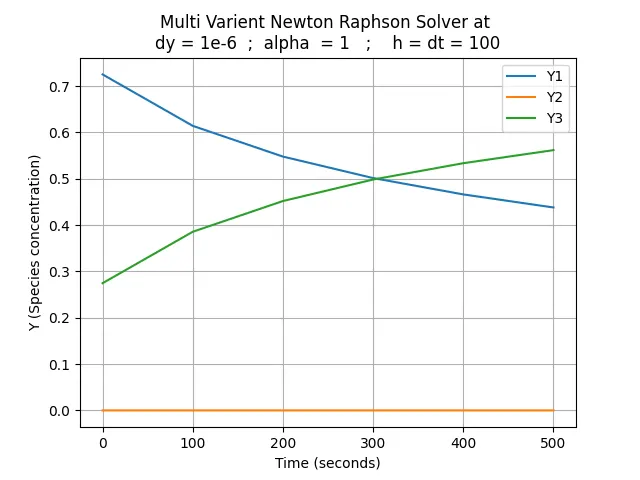
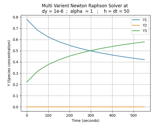
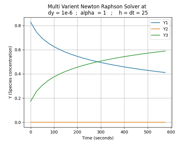
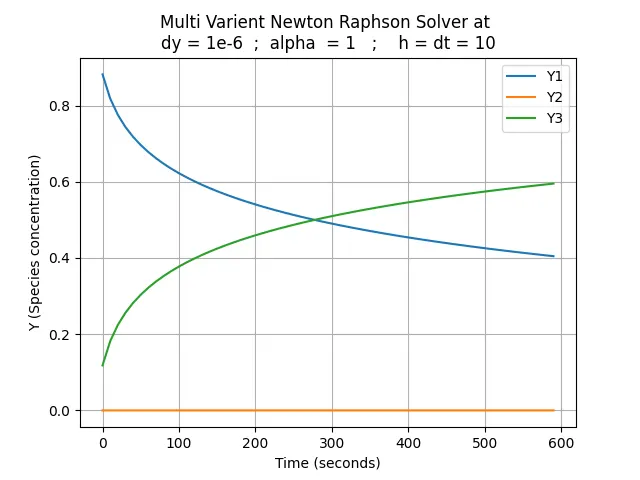
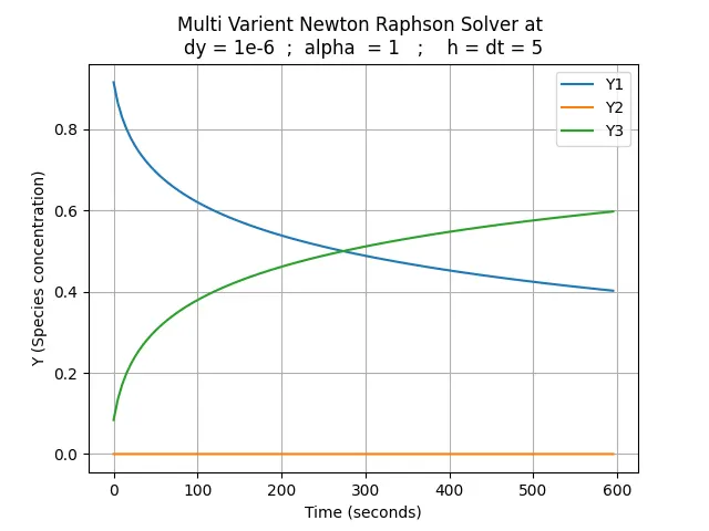
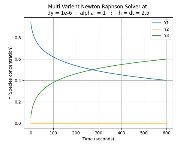
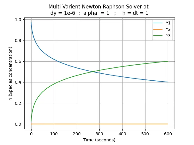
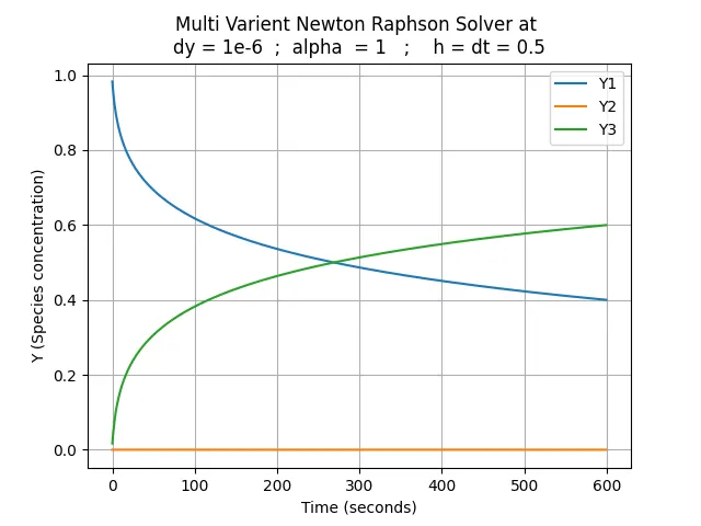
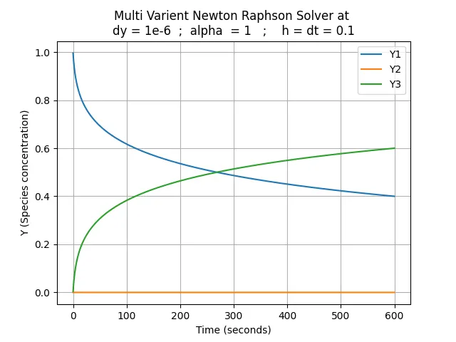
- Choose a suitable step size and explain the reason for choosing that step size, what is the ideal step size in this case?
|
Time step size `dt` |
Time taken to compute the results in seconds |
| 100 | 1.5 |
| 50 | 1.6 |
| 25 | 1.6 |
| 10 | 1.8 |
| 5 | 1.8 |
| 2.5 | 2 |
| 1 | 2.7 |
| 0.5 | 3.6 |
| 0.1 | 9 |
i computed the results for different step sizes `dt = [100,50,25,10,5,2.5,1,0.5,0.1]`
From the plots, we can understand that, as the step size decreases the solution is more smooth and accurate. For steps sizes, dt >10 the plots are not smooth and they are changing. step size dt < 10 plots are looking similar and exact as we reduce time step the plots remains same.
from the above table, we can notice that as the time step size decreases the time taken to compute the results also increases for dt = 100 it took 1.5 seconds to compute the results for dt = 0.1 it took 9 seconds to compute the results.
Reduced step size give accurate results but computation time increases by considering both the parameters accuracy and time taken to compute the results i recommend `1 > text(dt) >0.5`
NOTE:-
This Assignment is an example to solve the combustion mechanisms. in this, we considered 3 species `Y_1,Y_2,Y_3` as reference to analyzing how they are undergoing from reactants to products.
In real-time we will have 100,1000 species and reactions but the solution procedure is same as what we are doing here but, the scale of the problem will increase.
`text(Eample):-Y_1,Y_2,Y_3 == O_2,H_2O,C`