Week 6 - Multivariate Newton Rhapson Solver

During the combustion, lot of intermediary species are formed and their molar concentrations changes with time depending on temprature and pressure at that time. To estimate the emissions and thermodynamic properties of end products, whole reaction mechanism must be known. To get the reaction mechanism, reaction rates of each elemenrtary recation and production rate of each species formed during the combustion process must be calculated.

The reaction rate of a reaction and production rate of a species depends on molar concentration of other species. This results in a coupled non linear differential equations. These kind of coupled non linear equations can be solved using Multivariate Newton Rhapson method.

Multivariate Newton Rhapson Method:

let 'Y' be the value to be found (molar concentration of a particular species)

In this method, initially, a guess value for 'Y' is taken and iterated multiple times until it satisfies a particular condition. The value of 'Y' generated immeaidately afer satisfyitng the condition is the result.

``Y^(new) = `Y^(old) - (alpha*J^(-1)*F)` ---> (1)

where `alpha` is the relaxation factor.

For a system of equations, where `Y_1`, `Y_2` and `Y_3` are to be found,

Y1^(new) = `Y_1^(old) - (alpha*J^(-1)*F_1)` `

Y2^(new) = `Y_2^(old) - (alpha*J^(-1)*F_2)` `

Y3^(new) = `Y_3^(old) - (alpha*J^(-1)*F_3)` `

where `F_1, F_2 and F_3`are different functions of `Y_1`, `Y_2` and `Y_3` thus becoming coupled differential equations.

and 'J' is the Jacobi matrix which contains all the possible derivatives of functions `F_1, F_2 and F_3`.

`J = [[(delF_1)/(delY_1), (delF_1)/(delY_2), (delF_1)/(delY_3)], [(delF_2)/(delY_1),(delF_2)/(delY_2),(delF_2)/(delY_3)], [(delF_3)/(delY_1),(delF_3)/(delY_2),(delF_3)/(delY_3)] ]`

To find the values of `Y_1`, `Y_2` and `Y_3`, initially guess values for `Y_1`, `Y_2` and `Y_3` are taken and substituted for `Y_1^(old), Y_2^(old) and Y_3^(old)` respectively and values of Y1new, Y2new and Y3new are found. If these new values satisfy a particular condition(condition being the difference between old and new values to be very less approximately of the order `e^(-12)`). If the difference is more than the set value, the new obtained values are copied as old guess values for next iteration. Until the difference becomes less than set value, iterations continue and when it is less, the final `Y_1`, `Y_2` and `Y_3` are obtained.

In the given problem, the 3 coupled non linear ODEs are solved using the above method by applying implicit backward difference approach.

Discretizing the time derivative on LHS implicitly with backward difference,

`(y_1^n - y_1^(n-1))/dt = -0.04*y_1^n + 10^4*y_2^n*y_3^n`

`(y_2^n - y_12^(n-1))/dt = 0.04y_1^n - 10^4y_2^ny_3^n - 3*10^7*(y_2^2)^n`

`(y_3^n - y_3^(n-1))/dt = 3*10^7*(y_2^2)^n`

where `y_n`is the value of 'y' at time 'n' and

`y_(n-1)` is the value of 'y' at previous time 'n-1'.

RHS of above equations are `F_1, F_2 and F_3` respectively

Rearranging the above equations,

`y_1^(n-1) + dt*(-0.04*y_1^n + 10^4*y_2^n*y_3^n) - y_1^n = 0`

`y_2^(n-1) + dt*(0.04y_1^n - 10^4y_2^ny_3^n - 3*10^7*(y_2^2)^n) - y_2^n = 0`

`y_3^(n-1) + dt*(3*10^7*(y_2^2)^n) - y_3^n = 0`

The Jacobi matrix is evaluated at time step 'n'.

`J = [[((delF_1)/(delY_1))^n, ((delF_1)/(delY_2))^n, ((delF_1)/(delY_3))^n], [((delF_2)/(delY_1))^n,((delF_2)/(delY_2))^n,((delF_2)/(delY_3))^n], [((delF_3)/(delY_1))^n,((delF_3)/(delY_2))^n,((delF_3)/(delY_3))^n] ]`

The derivatives are evaluated numerically using Taylor series.

The first order approximation of taylor series,

`f'(y) = (f(y+dy) - f(y))/dy`

Applying the above formula for derivatives in Jacobi matrix,

`(delF_1)/(delY_1) = (F_1(Y_1+dy) - F_1(Y_1))/dy`

`(delF_1)/(delY_2) = (F_1(Y_2+dy) - F_1(Y_2))/dy`

`(delF_1)/(delY_3) = (F_1(Y_3+dy) - F_1(Y_3))/dy`

`(delF_2)/(delY_1) = (F_2(Y_1+dy) - F_2(Y_1))/dy`

`(delF_2)/(delY_2) = (F_2(Y_2+dy) - F_2(Y_2))/dy`

`(delF_2)/(delY_3) = (F_2(Y_3+dy) - F_2(Y_3))/dy`

`(delF_3)/(delY_1) = (F_3(Y_1+dy) - F_3(Y_1))/dy`

`(delF_3)/(delY_2) = (F_3(Y_2+dy) - F_3(Y_2))/dy`

`(delF_3)/(delY_3) = (F_3(Y_3+dy) - F_3(Y_3))/dy`

The above equations are substituted in Newton Rhapson equation and the code is written in Python. The simulation is made to run for 10 minutes. The values of `Y_1, Y_2 and Y_3` at time t=0 and guess values for getting convergence are both taken as 1, 0, 0 respectively. Relaxation factor is considered 1.

Value of 'dy' is taken 0.001 and time step size (dt) is varied.

Python Code:

"""
To solve a system of non linear coupled ODEs

dy1/dt = -0.04y1 + 10^4y2y3

dy2/dt = 0.04y1 - 10^4y2y3 - (3*10^7)y2^2

dy3/dt = (3*10^7)y2^2

Solving using multivariate Newton rhapson method

Y_new = Y_old - (alpha)*(inv J)*F

Jacobi is obtained by numerical derivative 

f'(y) = (f(y+dy) - f(y))/dy

"""

import math
import matplotlib.pyplot as plt 
import numpy as np 
from numpy.linalg import inv 

alpha = 1.0
dt = 0.01
dy = 0.001
tol = 1e-12
tot = 600
n = tot/dt
time_step = 0
t = np.linspace(1,tot,num=round(n))

# defining functions

def f1(y_prev1,y1,y2,y3,dt):

	return (y_prev1 + dt*(-0.04*y1 + pow(10,4)*y2*y3) - y1)

def f2(y_prev2,y1,y2,y3,dt):

	return (y_prev2 + dt*(0.04*y1 - pow(10,4)*y2*y3 - 3*pow(10,7)*pow(y2,2)) - y2)

def f3(y_prev3,y1,y2,y3,dt):

	return (y_prev3 + dt*(3*pow(10,7)*pow(y2,2)) - y3) 

# defining Jacobi

def Jacobi(y_prev1,y_prev2,y_prev3,y1,y2,y3,dt):

	J = np.ones((3,3))

	J[0,0] = (f1(y_prev[0],y_old[0]+dy,y_old[1],y_old[2],dt) - f1(y_prev[0],y_old[0],y_old[1],y_old[2],dt))/dy 
	J[0,1] = (f1(y_prev[0],y_old[0],y_old[1]+dy,y_old[2],dt) - f1(y_prev[0],y_old[0],y_old[1],y_old[2],dt))/dy 
	J[0,2] = (f1(y_prev[0],y_old[0],y_old[1],y_old[2]+dy,dt) - f1(y_prev[0],y_old[0],y_old[1],y_old[2],dt))/dy 

	J[1,0] = (f2(y_prev[1],y_old[0]+dy,y_old[1],y_old[2],dt) - f2(y_prev[1],y_old[0],y_old[1],y_old[2],dt))/dy 
	J[1,1] = (f2(y_prev[1],y_old[0],y_old[1]+dy,y_old[2],dt) - f2(y_prev[1],y_old[0],y_old[1],y_old[2],dt))/dy 
	J[1,2] = (f2(y_prev[1],y_old[0],y_old[1],y_old[2]+dy,dt) - f2(y_prev[1],y_old[0],y_old[1],y_old[2],dt))/dy 

	J[2,0] = (f3(y_prev[2],y_old[0]+dy,y_old[1],y_old[2],dt) - f3(y_prev[2],y_old[0],y_old[1],y_old[2],dt))/dy 
	J[2,1] = (f3(y_prev[2],y_old[0],y_old[1]+dy,y_old[2],dt) - f3(y_prev[2],y_old[0],y_old[1],y_old[2],dt))/dy 
	J[2,2] = (f3(y_prev[2],y_old[0],y_old[1],y_old[2]+dy,dt) - f3(y_prev[2],y_old[0],y_old[1],y_old[2],dt))/dy 

	return J

y1_final = []
y2_final = []
y3_final = []
iterations = []
y_prev =  np.zeros((3,1))  # initial conditions at time t=0
y_prev[0] = 1
y_old = np.zeros((3,1)) # guess values
y_old[0] = 1
F = np.copy(y_old)

# Time loop

for i in range(0,round(n)):

	error = 9e9
	time = dt*time_step
	iter = 0

	while error > tol:

		J = Jacobi(y_prev[0],y_prev[1],y_prev[2],y_old[0],y_old[1],y_old[2],dt)

		F[0] = f1(y_prev[0],y_old[0],y_old[1],y_old[2],dt)
		F[1] = f2(y_prev[1],y_old[0],y_old[1],y_old[2],dt)
		F[2] = f3(y_prev[2],y_old[0],y_old[1],y_old[2],dt)
		y_new = y_old - alpha*np.matmul(inv(J),F)

		error = np.max(np.abs(y_new-y_old))

		y_old = y_new 
		iter = iter + 1

	print(iter)
	y_prev = y_old
	y1_final.append(y_prev[0])
	y2_final.append(y_prev[1])
	y3_final.append(y_prev[2])
	iterations.append(iter)

	log_message = 'time = {0} y_prev1 = {1} y_prev2 = {2} y_prev3 = {3}'.format(time,y_prev[0],y_prev[1],y_prev[2])
	print(log_message)
	time_step = time_step + 1

plt.figure()
plt.plot(t,y1_final,color='red')
plt.plot(t,y2_final,color='blue')
plt.plot(t,y3_final,color='green')
plt.legend(['Y1','Y2','Y3'])
plt.xlabel('time')
plt.ylabel('Y')
plt.show()

plt.figure()
plt.plot(t,iterations)
plt.xlabel('time')
plt.ylabel('No. of iterations to get convergence for each time step')
plt.show()

Values of previous time step ( at 'n-1' time step) are given in array 'y_prev'

Guess values are given in array 'y_old'.

The time step size is taken 0.01.

The functions `F_1, F_2 and F_3` and Jacobi matrix are defined.

A time loop is created that iterates from time t=0 to 600 seconds.

A convergence loop inside time loop is created which gives values of `Y_1`, `Y_2` and `Y_3` for each time step.

After every time step, values of `Y_1`, `Y_2` and `Y_3` are stored in array 'y_prev' as it would become previous time step values for next time step.

Results:

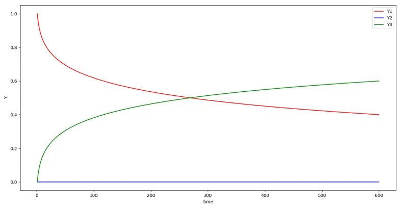
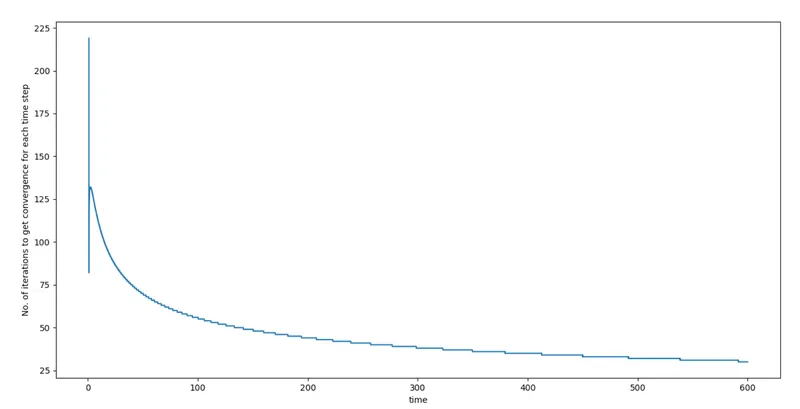
1. For dt = 0.01, no. of time steps to complete simulation for 10 mins would be 60000.

Values of `Y_1`, `Y_2` and `Y_3` after 10 mins are obtained as

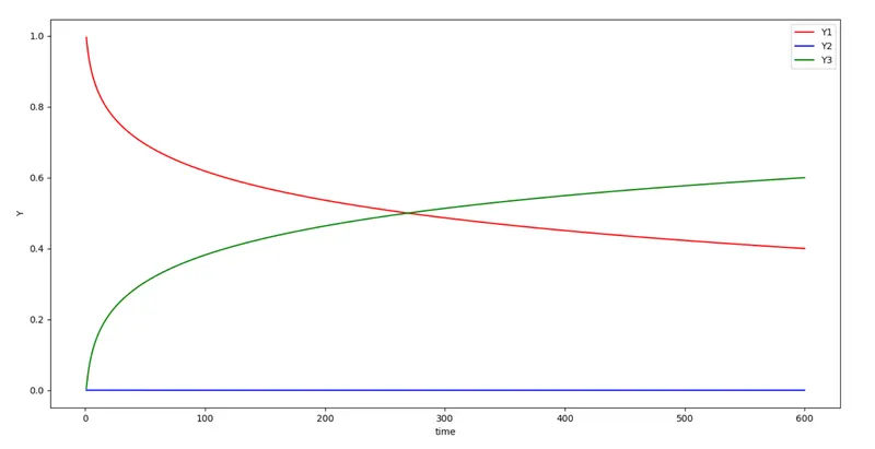
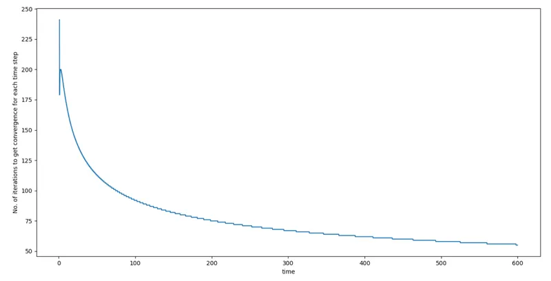
2. For dt = 0.1, no. of time steps to complete simulation for 10 mins would be 6000.

Values of `Y_1`, `Y_2` and `Y_3` after 10 mins are obtained as

No. of iterations to get convergence for each time step:

Conclusions:

From the above plots, it is observed that the values of `Y_1`, `Y_2` and `Y_3` does not change with change in time step size and also the results are stable.

This is the advantage of using implicit approach. The result will be stable irrespective of time step size. So, time step size need not be small to get stable results. Bigger time step size can be used so as to get results faster.

But there is a constraint to be considered. The combustion process happens in a very short time (order of micro seconds) i.e., within the duration of just micro seconds, there will be a lot of different species formed and their concentrations might change in a rapid pace. If the chnage in species concentration needs to be observed, then the simulation must be made to run with a very small time step size. Then the change can be observed more clearly. With this information, one can understand how the concentration of a species is changing and at what time a particular species is reacting with other species. The reaction map is obained accurately and thereby the emissions and thermodynamic properties of products can be predicted with good accuracy.

Also, it is observed that with a smaller time step, no. of iterations taken by newton rhapson method to attain convergence for each time step is less but the total time to simulate will be higher.