Week 6 Fuel cell powered vehicle model
MATLAB model of fuel cell powered electric vehicle
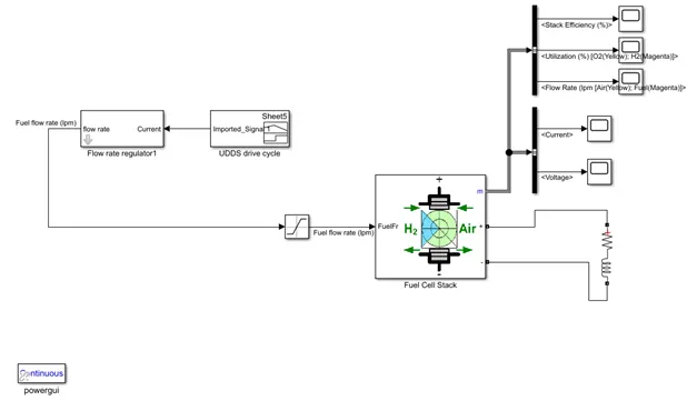
Figure 1: MATLAB model for a fuel cell powered Electric Vehicle
The MATLAB model for fuel cell powered electric vehicle is as shown in figure1. This model consists of the following blocks.
- UDDS drive cycle
- Flow rate regulator
- Fuel cell stack
- UDDS drive cycle
The input to the fuel cell model is the UDDS cycle. But we haven’t implemented driver and vehicle model to get the desired current for corresponding velocity. So we have to input the current profile to the signal builder block in order to generate corresponding signals. The time and current data can be imported to signal builder block from excel sheet. We get the following signal after importing UDDS current profile.
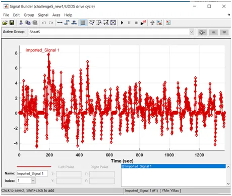
Figure 2: UDDS current signals in signal builder
- Flow rate regulator
This block will convert the current to corresponding flow rate of the fuel. The relation between flow rate and fuel cell current is expressed by the following equation.
Uf_H2 =
where
Pfuel = absolute supply pressure of fuel (atm)
Vfuel = fuel flow rate (l/min)
Vair = air flow rate (l/min)
x = percentage of hydrogen in the fuel (%)
R = 8.3145 J/(mol K)
Nc = No.of cells
96485 = Faraday’s constant A s/mol
z = number of moving electrons (z = 2)
Air outlet pressure = 101325
From the bove equation, following equation has been derived.
Vfuel =60000*R*(273+T)*Nc*i_fc/(2*96485*(Pfuel*101325)*Uf_H2/100*x/100)
This equation will convert current to corresponding fuel flow rate.
- Fuel Cell Stack
This block implement generic hydrogen fuel cell stack model and it can be accessed from the following library in MATLAB.
Simscape / Electrical / Specialized Power Systems / Electric Drives / Extra Sources
Description
The Fuel Cell Stack block implements a generic model parameterized to represent most popular types of fuel cell stacks fed with hydrogen and air.
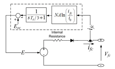
Figure 2: Simplified Model
The block represents two versions of the stack model: a simplified model and a detailed model. We can switch between the two models by selecting the level in the mask under Model detail level in the block dialog box.
The simplified model represents a particular fuel cell stack operating at nominal conditions of temperature and pressure. The parameters of the equivalent circuit can be modified based on the polarization curve obtained from the manufacturer datasheet. You just have to input in the mask the value of the voltage at 0 and 1 A, the nominal and the maximum operating points, for the parameters to be calculated. A diode is used to prevent the flow of negative current into the stack. Figure 2 represents simplified model of fuel cell.
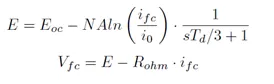
------------------------ (1) & (2)
where
Eoc = open circuit voltage (V)
N = number of cells
A = Tafel slope (V)
i0 = exchange current (A)
Td = the response time (at 95% of the final value) (sec)
Rohm = internal resistance ()
ifc = fuel cell current (A)
Vfc = fuel cell voltage (V)
In a sudden change in stack current, the fuel cell voltage will exhibit a delay which is approximately 3 times the time constant (τ = RC) prior to equilibrium. This phenomenon is represented in equation (1) by delaying the activation losses with a first order transfer function 1/(sTd/3+1) with Td being the stack settling time.
Equation (2) gives the stack total voltage considering the losses due to electrodes and electrolyte resistances (ohmic losses). The simplified model can be used to simulate fuel cell stacks operating at nominal condition of temperature and pressure. A diode is used to prevent the flow of negative current into the stack.
- The detailed model
The detailed model represents a particular fuel cell stack when the parameters such as pressures, temperature, compositions and flow rates of fuel and air vary. These variations affect the Tafel slope (A), the exchange current (i0) and the open circuit voltage (Eoc). The equivalent circuit of the detailed model (shown in Fig. 2 ) is the same as for the simplified one, except that the parameters (Eoc, i0, A) will have to be updated based on the input pressures and flow rates, stack temperature and gases compositions.
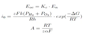
-------------------------- (3), (4) , (5)
Eoc, i0 and A are modified as follows [3], [7]:
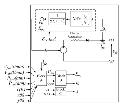
Figure 3: Detailed model
where
R = 8.3145 J/(mol K)
F = 96485 A s/mol
z = number of moving electrons (z = 2)
En = Nernst voltage (V)
_ = charge transfer coefficient
PH2 = partial pressure of hydrogen inside the stack (atm)
PO2 = partial pressure of oxygen inside the stack (atm)
k = Boltzmann’s constant (1.38×10⁻²³ J/K)
h = Planck’s constant (6.626×10⁻³⁴ J s)
_G = activation energy barrier (J)
T = temperature of operation (K)
Kc = voltage constant at nominal condition of operation
As shown in Fig. 2, new values of Eoc, i0 and A are calculated using Block A, B and C. At first, the rates of conversion (utilizations) of hydrogen (UfH2 ) and oxygen (UfO2 ) are determined in Block A as follows:
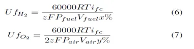
where
Pfuel = absolute supply pressure of fuel (atm)
Pair = absolute supply pressure of air (atm)
Vfuel = fuel flow rate (l/min)
Vair = air flow rate (l/min)
x = percentage of hydrogen in the fuel (%)
y = percentage of oxygen in the oxidant (%)
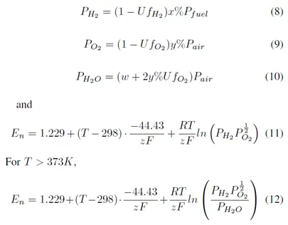
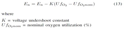
Knowing the partial pressures of gases and the Nernst voltage, the new values of the open circuit voltage and the exchange current can therefore be calculated using equation (3) and (4) respectively. Block C calculates the new value of the Tafel slope using equation (5). The effect of oxygen depletion (due to the air compressor delay) on the stack voltage can be modeled if the parameters for flow dynamics such as the peak utilization (UfO2(peak)) and the corresponding voltage undershoot (Vu) are known. The lack of oxygen inside the cell causes its utilization to increase above the nominal value and the Nernst voltage will be modified as follows:
Data extraction and model parameters approximation Fuel cell manufacturers provide specifications1 of their stacks which include the polarization curve, rated and peak power, number of cell, efficiency, temperature, inlet pressures, etc. These data are used to obtain the models parameters. 1) Data required from datasheet: For the simplified model, four parameters (Eoc, i0, NA and Rohm) are to be determined, which requires at least four simultaneous equations. Two points from each region (activation and ohmic) are taken on the polarization curve as shown in Fig. 3. These points correspond to the following:
- Current and voltage at nominal operating point: (Inom, Vnom)
- Current and voltage at maximum operating point: (Imax, Vmin)
- Voltage at 0 and 1 A: (Eoc, V1)
For the detailed model, in addition to (Eoc, i0, NA and Rohm), four more parameters (_, _G, K, Kc ) are to be determined. Therefore, in addition to the four points on the polarization curve, the following variables are needed:
- Number of cells in series (N)
- Nominal LHV stack efficiency (_nom) in %
- Nominal operating temperature (Tnom) in oC
- Nominal air flow rate (Vair(nom)) in liter/min
- Absolute supply pressures (Pfuel(nom), Pair(nom)) in atm
- Nominal composition of fuel and air (xnom, ynom, wnom) in %
To represent accurately the fuel cell dynamics, current step and interrupt tests must be made on a real stack. Fig. 4 shows the stack response from these tests and the required parameters (Td, UfO2(peak) and Vu ). The response time (Td) depends on the fuel cell stack itself and is usually given on the datasheet. The parameters for flow dynamics (UfO2(peak) and Vu) depend on the dynamics of external equipments (compressor, regulator and loads) and they are not provided by manufacturers as their values vary with the user application. For simulation, the user may assume values of UfO2(peak) between 60-70 %2 and Vu between 2-5 % of the stack nominal voltage.
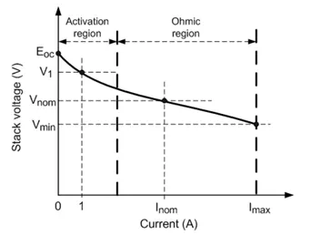
Figure 4: Typical polarization curve
- Data Extraction from datasheet
A model of a 6.8kW-230V, PEMFC stack (Nedstack FCS 7-XXL) from NedStack is made using its datasheet. The following values are extracted from the datasheet:
- Voltage at 0 A and 1 A [Eoc, V1] = [46.6, 44]
- Nominal operating point [Inom, Vnom] = [120, 34.7]
- Maximum operating point [ Imax, Vmin] = [230, 29.5]
- Nominal stack efficiency (_nom) = 55 %
- Number of cells in series (N) = 48
- Operating temperature = 65 oC
- Nominal air flow rate (Vair(nom)) = 190 liter/min
- Nominal composition of fuel and air [xnom, ynom, wnom] = [99.999, 21, 1]
- Nominal supply pressure [H2, Air] = [1.5 1]
The polarization curve from datasheet is shown in figure 5. Figure 6 shows the polarization curve plotted from MATLAB model. We can see that the model almost behaves like datasheet values.
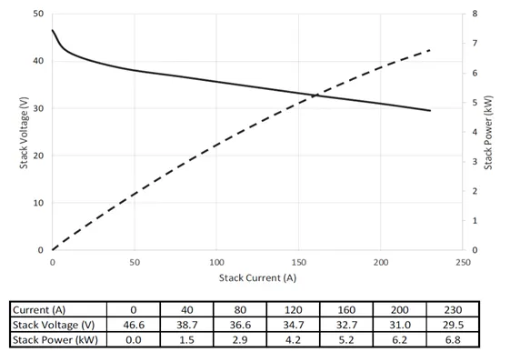
Figure 5: Polarisation curve from datasheet
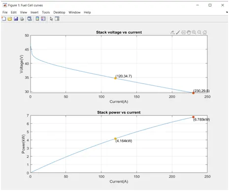
Figure 6: Polarisation curve from MATLAB model
Analysis of Results
Figure 7 to Figure 12 shows the output plots of fuel cell powered electric vehicle. Figure 7 shows UDDS cycle. The positive current shows the acceleration and negative currents shows braking. Fuel supplies power when current demand is positive (during acceleration).
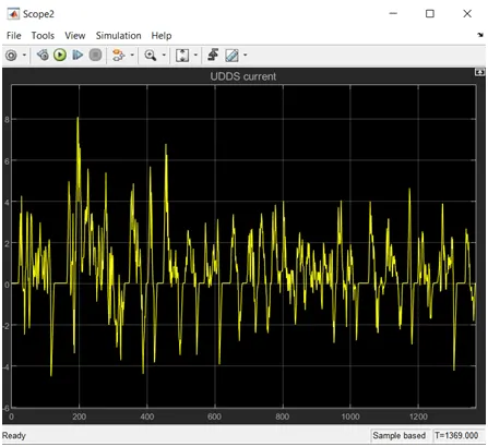
Figure 7: UDDS current plot
Fuel cell won’t respond to immediate changes in the current because of the delay introduced to it. This we can observe from fuel cell current plot. The stack efficiency is expected to be 55% during operating region. But because of the sudden load changes, it follows the figure 8 plot.
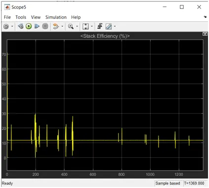
Figure 8: Stack Efficiency plot
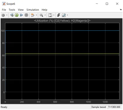
Figure 9: Fuel and Air Utilization
The fuel flow rate is shown in blue plot and air flow rate is shown in yellow plot. From figure 10, we can see that there will be a continuous flow of fuel irrespective of the load demand.
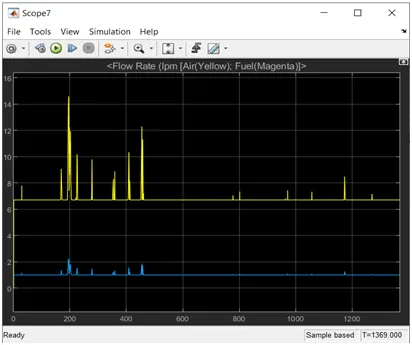
Figure 10: Fuel and Air flow rate
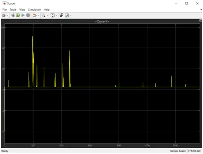
Figure 11: Fuel cell Current
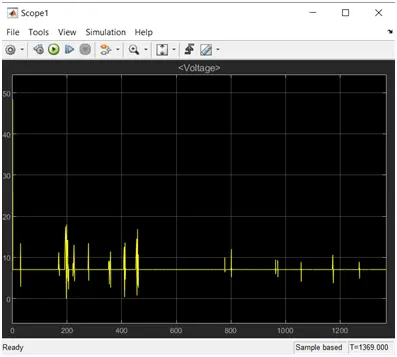
Figure 12: Fuel cell Voltage
The fuel cell current and voltage plots are shown in figure 11 and 12. We can see that there will be continuous flow of current irrespective of load demand. And fuel cell won’t shut down even if the load demand is zero.
Conclusion
The MATLAB model of fuel cell powered electric vehicle has been simulated and behavior of Fuel cell has been analysed for UDDS drive cycle.
The MATLAB model and fuel cell datasheet has been attached