Data analysis PYTHON

AIM

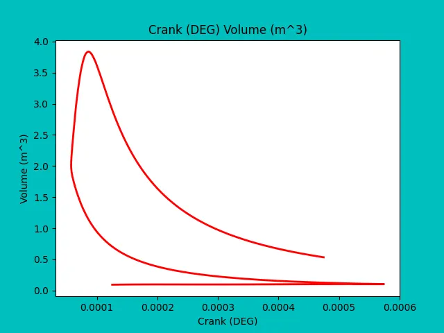
• Calculate the area under the P-V diagram. P is in column 2 and V is in column 8.
• Calculate the power output of this engine. Assume that RPM is 1500
• This engine consumed 20 micro grams of fuel (per 1 stroke cycle). Calculate its specific fuel consumption.

Above objectives should be achieved by python programming.

THEORY:

Power output of the Engine:

power = workdone/time

power = w*2*π">π*n

= w*2*π">π*N/60

where,

P is power in KW

n is speed(rev/s)

N is speed(RPM)]

Specific Fuel consumption:

SFC is the amount of fuel consumed by engine for each unit of power output.

SFC = 3600*mf*n/power

= (mf*N)/60*P

CODE:

import math
import matplotlib.pyplot as plt
import numpy as np
from scipy.optimize import curve_fit
from scipy.integrate import simps, trapz as trapz


file = 'engine_data.out'

try:
	open(file)
except:
	print('File not recognized. Please provide a valid CONVERGE output file')
else:
	ct = 1

	x = []
	y = []

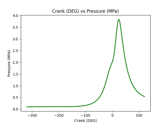
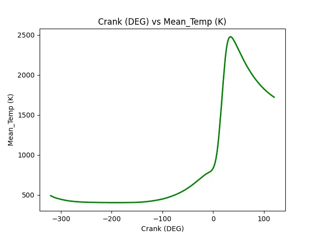
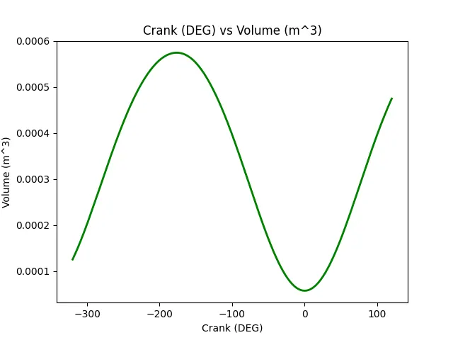
	a = int(input('x variable:  '))
	b = int(input('y variable:  '))
	for line in open(file):

		if '#' not in line:
			x.append(float(line.split()[a-1]))
			y.append(float(line.split()[b-1]))

		if ct == 3:
			tempx= line.split()[a]
			tempy= line.split()[b]

		if ct == 4:
			labelx = ('%s %s' %(tempx, line.split()[a]))
			labely = ('%s %s' %(tempy, line.split()[b]))
			print('X_Axis variable:', labelx)
			print('Y_Axis variable:', labely)

		ct+=1

plt.figure(1)
plt.plot(x,y, linewidth = 2, color = 'green')
plt.title('%s vs %s' %(labelx,labely))
plt.xlabel('%s' %labelx)
plt.ylabel('%s' %labely)
plt.savefig('%s vs %s' %(tempx,tempy),facecolor = 'y')
plt.show()

    #calculation

ct = 1
p_c = 2
p = []
v_c = 8
v = []

for line in open(file):
    if '#' not in line:
    	p.append(float(line.split()[p_c - 1]))
    	v.append(float(line.split()[v_c - 1]))
    if ct == 3:
    	tempx =  line.split()[v_c]
    	tempy = line.split()[p_c]
    if ct == 4:
    	labelx = ('%s %s' %(tempx, line.split()[v_c]))
    	labely = ('%s %s' %(tempy, line.split()[p_c]))
    	ct+=1

plt.figure(2)
plt.plot(v,p, linewidth = 2, color = 'red')
plt.title('%s %s' %(labelx,labely))
plt.xlabel('%s' %labelx)
plt.ylabel('%s' %labely)
plt.savefig('%s vs %s' %(tempx,tempy), facecolor = 'c')
plt.show()

#trapezoidal for data sample:
A_t = trapz(p,v)
print('Area under PV diagram by trapezoidal rule is', A_t)
#simpson's rule for data sample:
A_i = simps(p,v)
print('Area under PV diagram by integration rule is', A_i)

N = 1500 #RPM
f_c = 20*pow(10,-6) # micro gram, per cycle =>> {f_c*(N/60)} is fuel consumption per hour

work = A_i*pow(10,6)
print('work done is %f (J)' %work)

power = (2*math.pi*N*work)/60
power = power/1000
print('power output of the engine is %f (kW)' %power)

#Specific fuel consumption cal:

spc = (f_c*(N*60))/(power)
print('Specific fuel consumption of the engine is %f (g/KW-h)' %spc)

RESULT:

x variable:  1
y variable:  8
X_Axis variable: Crank (DEG)
Y_Axis variable: Volume (m^3)
Area under PV diagram by trapezoidal rule is 0.0005005866274680075
Area under PV diagram by integration rule is 0.0005005864474262364
work done is 500.586447 (J)
power output of the engine is 78.631935 (kW)
Specific fuel consumption of the engine is 0.022891 (g/KW-h)
>>> 

IMAGES: