Creating connection for Rear door
AIM-
For the given Rear door FE model, create and apply different PIDs for different components and perform suitable connections.
To write a detailed report on why we choose a certain type of element for connecting certain parts of the door.
PROCEDURE -
The given model for deploying the connections is a side door of the car as shown in the below images. We import the same from the link given.
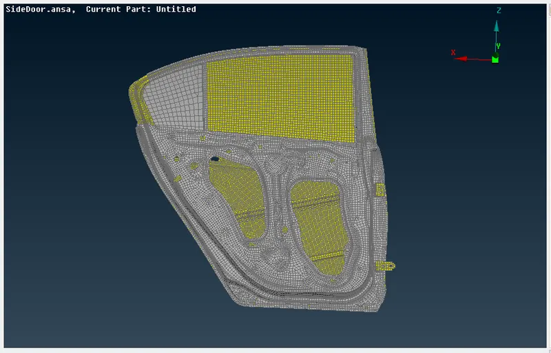
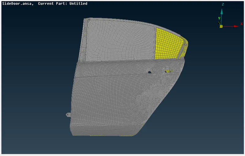
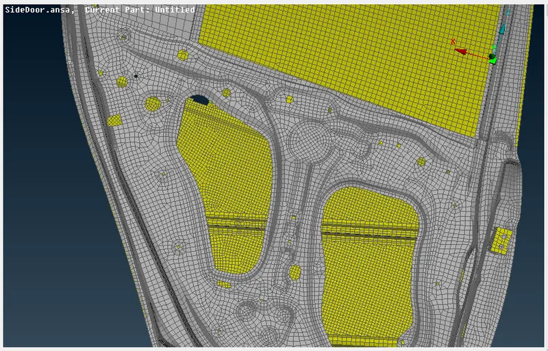
The model as shown above is the FE part of the side door and we need to work on it in this challenge.
The model when viewed in PID mode shows us that the model is in the same PID with the same color as shown below.
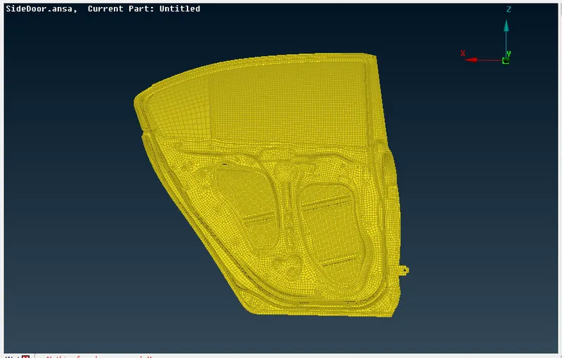
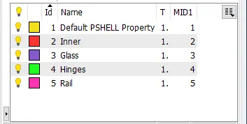
To deploy the connections, an entire model needs to be separated into different PIDs. Based on the components, the entire model is separated and will be named in the database window.
The new PID is assigned so that we can easily differentiate the type of components in the side door based on colors, the updated model is shown below.
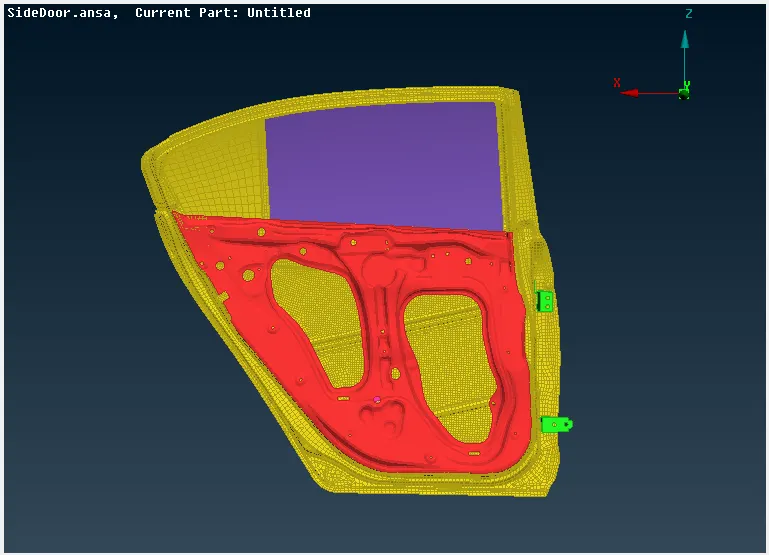
Each component with different color is assigned a different PID as shown in the image below.
STEP-1: Deploying the connections at hinges
Initially, the connections will be deployed at the hinge regions which connect the door to the car. The hinges in the model are shown below.
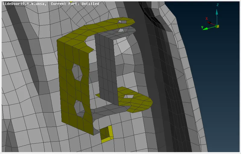
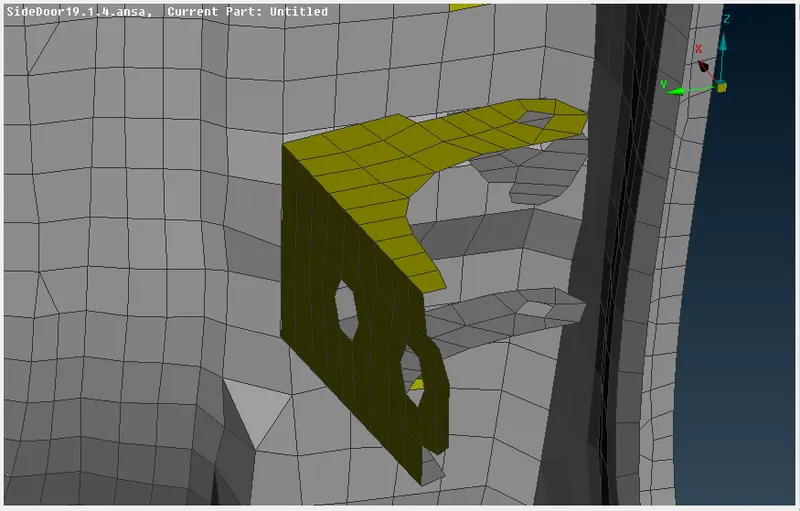
At the hinges, the bolted joint is used in the real scenario. For creating a bolt connection, a COG point is required which can be obtained by going to Topo module->Points->On COG. Select any one of the closer perimeters to obtain the COG as shown below.
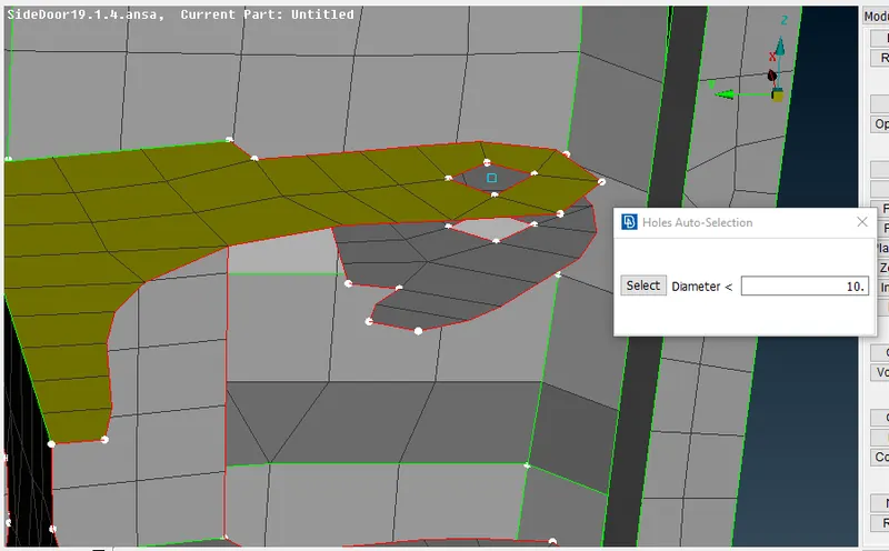
Now, we convert the COG which is created to a 3D point from the 'Convert' Option in the assembly manager.
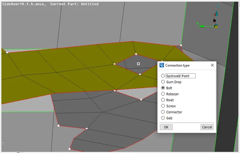
The 3D point (COG) is selected and the bolt option is chosen to convert the 3D point to a bolt. After this, the bolt will be represented as a hexagonal-shaped bolt.
Now, we use the 'Connection' option from the assembly manager and a dialog box appears.
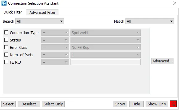
We confirm the procedure and then a new dialog box appears as shown below. Here, we need to define the P1 and P2 for the bolt connection. We need to right-click on P1 and press 'F1', we then select the area associated with P1 and then do the same for P2.
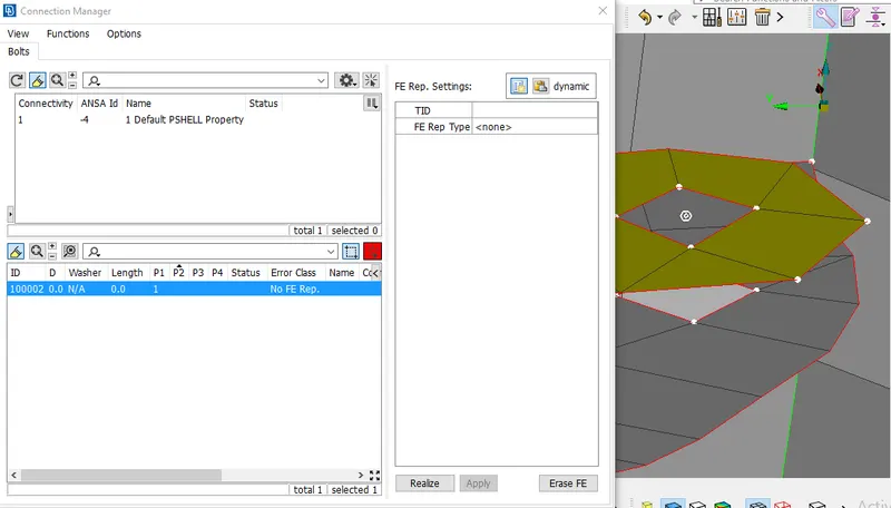
After defining P1 and P2, we select the FE Rep type to be 'Bolt' and then add the other requirements if needed. In this case, we will fix the 'search on direction' to be 10.
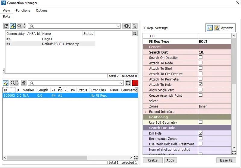
The next step is to apply the changes done and realize them. The result is shown below.
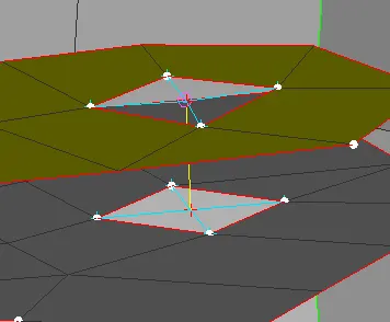
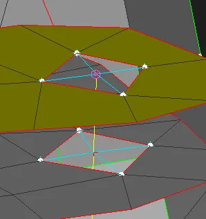
With the realization of the bolt connection, we will look into connecting hinges. Here, we go to NASTRAN deck->Elements->RBE2->Two nodes option and then select the required nodes.
The dialogue box will appear as shown below.
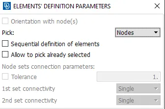
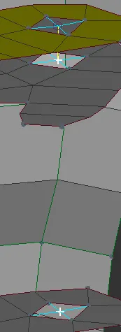
We proceed with selecting the 2 nodes between which a connection has to be established as shown in the image below.
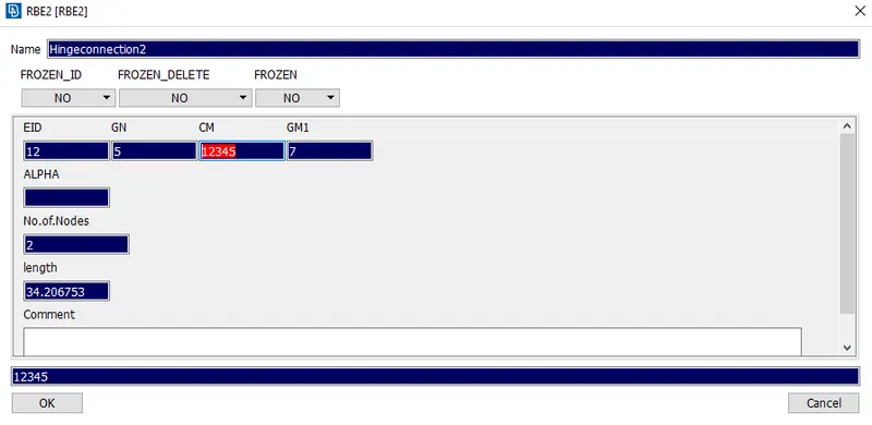
After confirmation of the selection of nodes, a dialog box appears which shows us the info about RBE2 elements. Here, we should constrain all directions except the rotation in Z-direction as the door will be moved in rotation to Z-axis. We can do this by changing the CM from 123456 to 12345 as shown below.
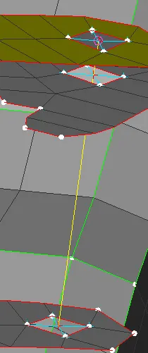
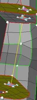
We then click on 'OK' and the RBE2 element with 2 nodes is created and is represented by the 'Yellow' line as shown below.
STEP-2: Deploying the connections with RBE2 elements
The RBE2 elements are deployed at some regions with the 'many nodes option'.
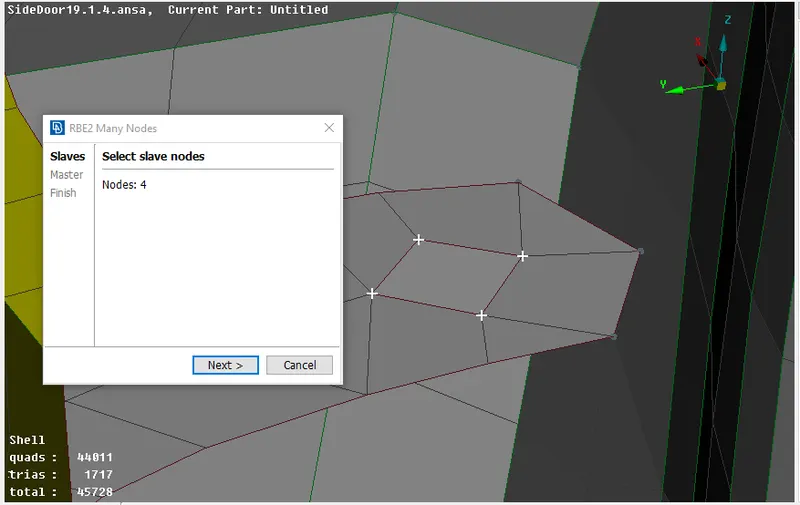
We go to 'NASTRAN deck->Elements->RBE2->Many nodes', a dialog box will open as shown below. We need to select the slave nodes as shown below.
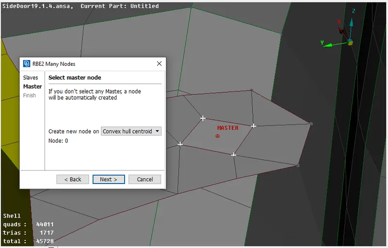
After confirming the slave nodes, we click on next and the tool will choose the master node itself based on the slave nodes that are selected as shown in the image below.
We click on next and the 'create entity' dialog box appears, here we can set the EID, the number of nodes, the degrees of freedom, and then we can click on finish.
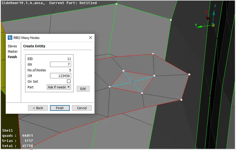
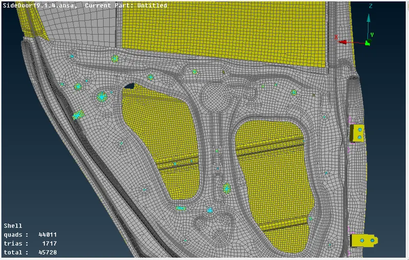
We can see in the above image that the connection has been created in the selected region, similarly, we do the same and define connections at various other regions in the model.
STEP-3: Deploying a connection at the door handle
The connection to be deployed is at the door handle region shown in the below image.
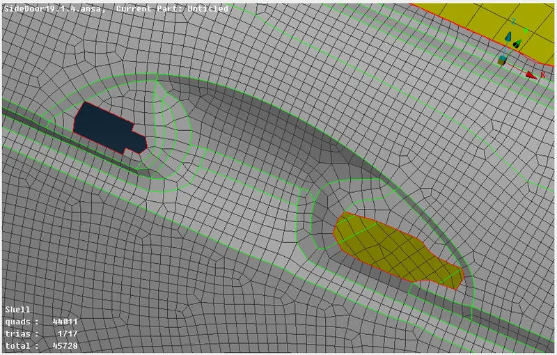
Initially, we define a connection using RBE2 elements with 'many nodes option' as shown in the image following the method explained in step 2.
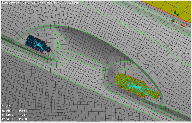
We then use the RBE2 element with many nodes to connect both the master nodes which is shown in the above image. The reason we use RBE2 with many nodes rather than 2 nodes is to have a master node after connecting the 2 master nodes. If we use the RBE2 with 2 nodes, there will be no master nodes after connecting those 2 portions.
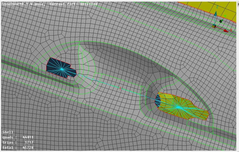
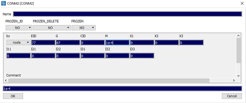
We now need to represent the weight of the door handle which is the case in the real-world scenario. The mass can be assigned by going to 'NASTRAN deck->Elements->CONMi->CONM2->Nodes'.
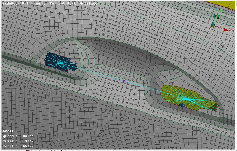
We now need to select the master node in between the door connection to add the weight which is shown in the image below.
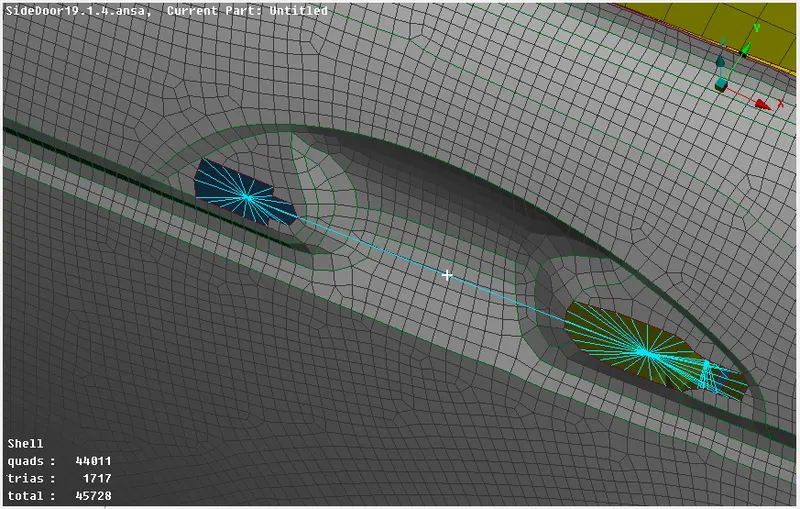
A weight of 1 kg is assumed for the door handle and a value of 1e-4 is put into the dialogue box (Kg to Tonnes).
After assigning the mass at the master node, it will be highlighted as shown in the image below.
STEP-4: Deploying a connection at the latch region
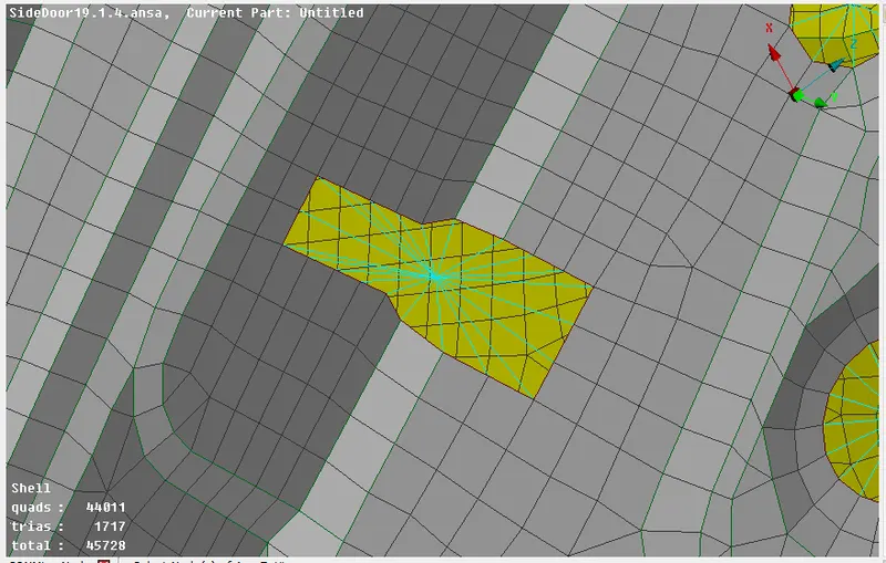
We use the RBE2 element for the connection. We go to 'NASTRAN->Elements->RBE2->Many nodes.
STEP-5: Deploying a connection between the rail and side glass:
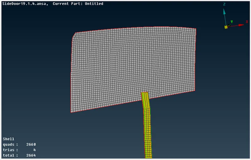
In this step, the rail which is responsible for the movement of side glass is isolated as shown in the below image.
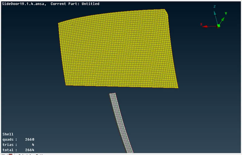
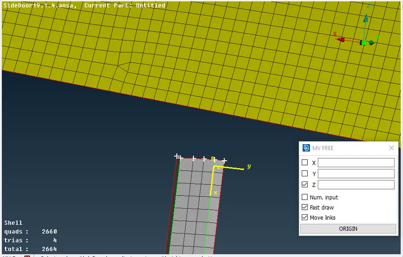
We can see that the rail component should be extended to the glass. This can be done by going to Mesh deck->Grids->MV Free. A new dialog box will open, we select the Z-axis as we need to move the rail in that direction and then select the nodes as shown below.
After extending the rail, it will look like the image shown below.
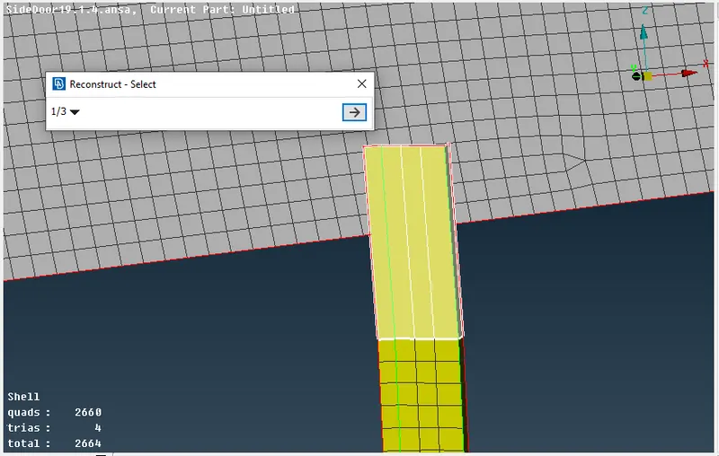
The mesh will be reconstructed in the rail as we can see the difference in the above image.
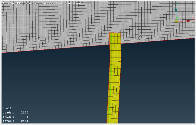
The part after reconstruction will look like the below image.
These 2 components are connected using the RBE2 elements as in the above steps. The connection defined is shown in the image below.
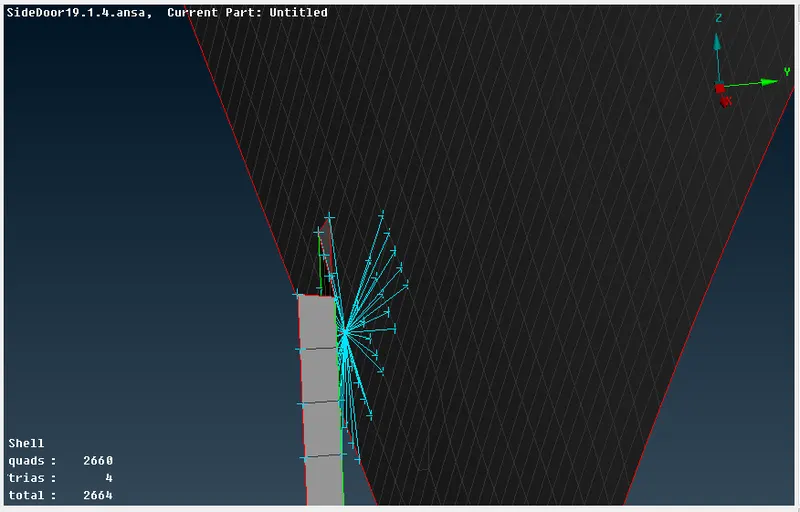
STEP-6: Deploying connections using the spot weld and seam weld
In some regions in the model, the parts have minimal space for them to be joined, so we join them by using the spot weld and seam weld option.
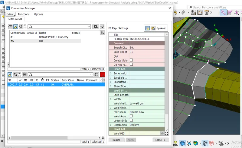
First, we create a curve where we perceive to start the seam weld and then convert the seam curve using the convert option. We open the connection manager and select P1 and P2, we select the FE Rep type as OVERLAP-SHELL (for parallel parts) or Y JOINT SHELL (for perpendicular parts). We then set an appropriate search distance and root shells and then realize the connection as shown in the below image.
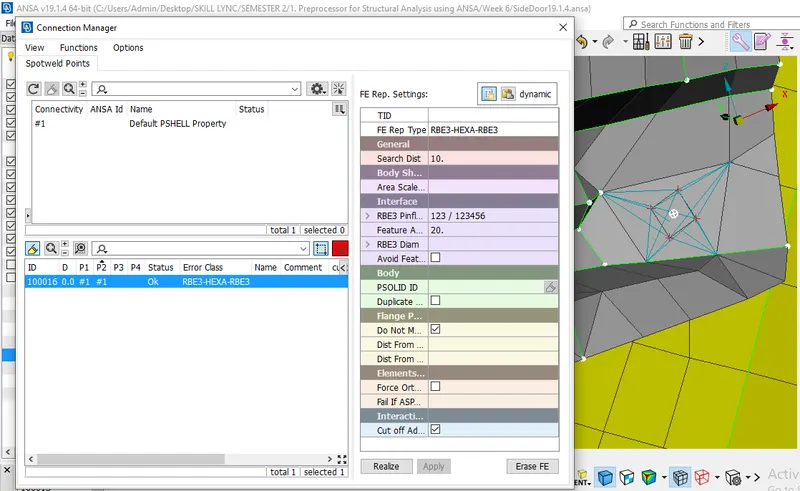
To create a spot weld, we create a 3D point at the center of the element. We then convert the point into a spot point using the convert option and then we open the connection manager and assign the required P1 and P2. We select the FE Rep type as RBE-HEXA-RBE3, insert the appropriate search distance and then realize the connection as shown in the image below.
STEP-7: Deploying a connection at the side glass region
The component surrounding the side glass is called a weather strip which is made up of rubber material and is widely known as beading. To represent that, we will be using the CBUSH elements as it possesses the elasticity in all 3 directions.
So, initially, the curves are needed and we can get this by using the 'Feat2Curve' option by going to Topo deck->Perimeters->Feat2curve. This is shown in the image below.
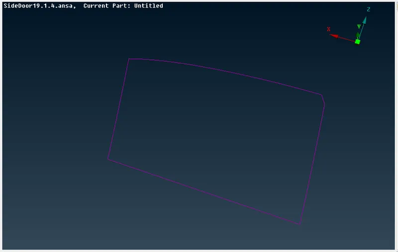
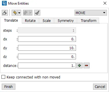
The weatherstrips will be at both sides of the glass at the bottom, the CBUSH elements should be deployed at the sides of the bottom. The curve at the bottom should be copied by using 'Transform' and moved to a distance of 10 mm (an assumption).
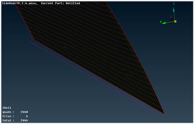
After copying and moving, the copied curve appears as shown in the image below.
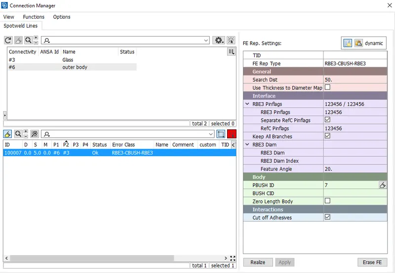
Now, we need to convert these curves into "Spot line". This spot line is realized by selecting line by line and specifying the parameters. The parameters are listed down below.
1. Spacing between CBUSH elements should be 10 mm
2. Specifying PART1 and PART2
3. Specifying FE representation type as '"RBE3-CBUSH-RBE3"
4. Assigning RBE3 pin flags (DOF) in all directions.
The connection manager window is shown below.
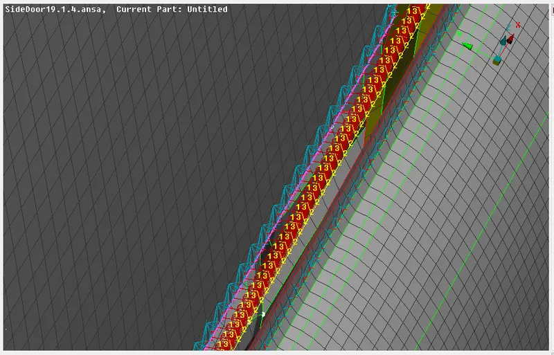
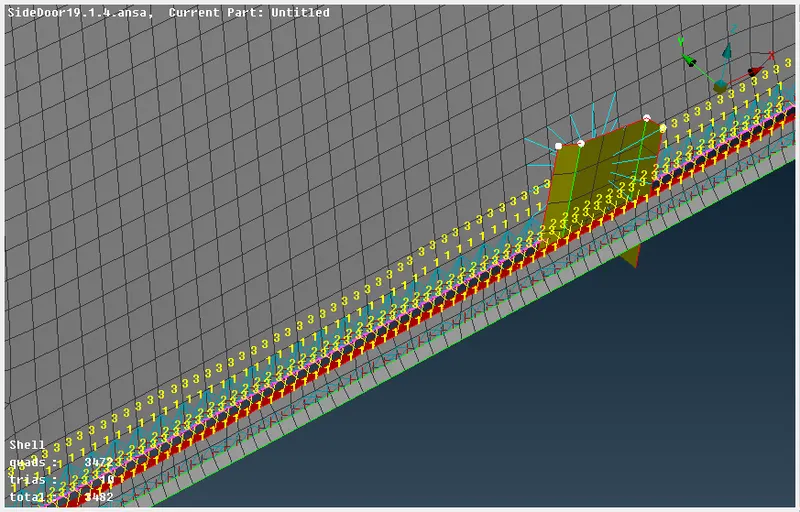
After this, we realize the CBUSH elements and we can see the element appearing as shown below.
Similarly, the CBUSH elements are created on all sides of the glass. After this, we isolate the elements and we can observe that the orientation is different.
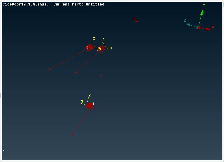
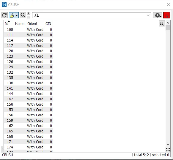
We enable all the CBUSH elements by selecting the option in the drop-down list. The list should include the CID and the orientation.
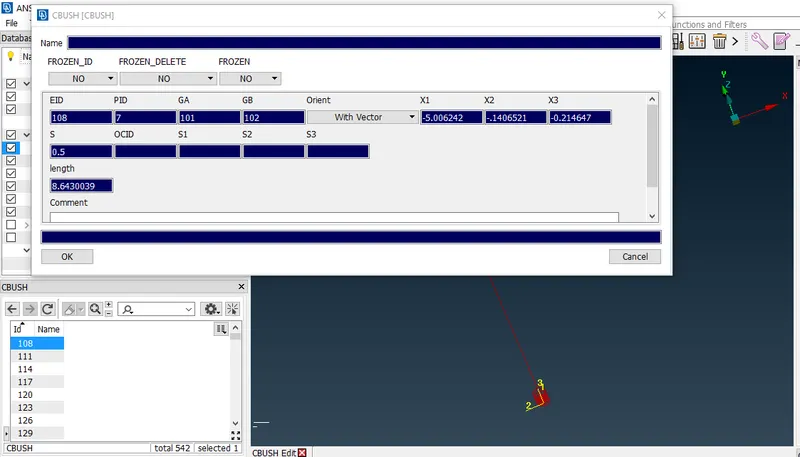
Here, we need to change the 'Orient' from 'with vector' to 'with coordinate' and give a value of 0 to CID. As there are many CBUSH elements in the model, we can't change the orientation one by one, so we select all the elements at once and right-click on the list, and click on modify.
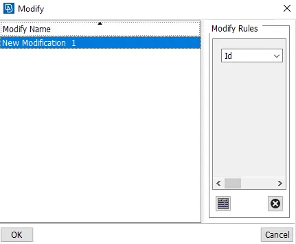
Now, from the drop-down list select 'Orient' and 'with Cord'. Next, select 'CID' and then dd the value '0'.
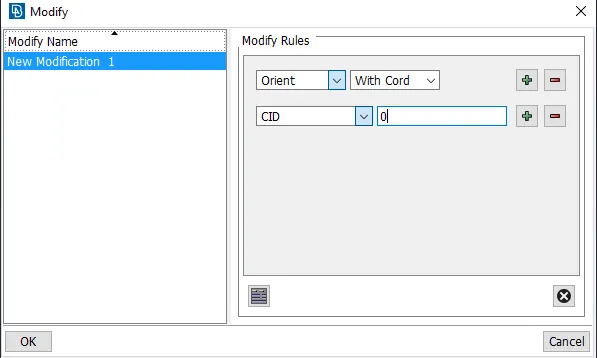
We click 'OK' and confirm the selection. This will orient all the CBUSH elements with the global coordinates as shown below
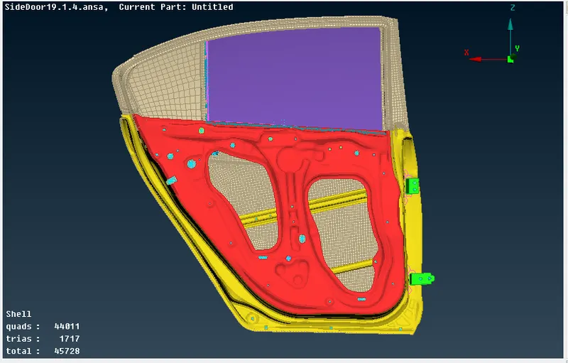
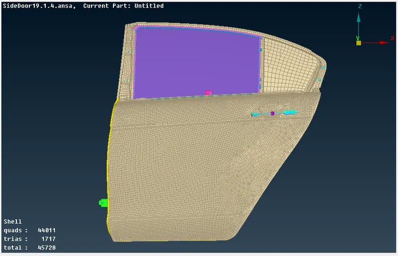
With this, all the important connections are defined in the model and are shown below.
CONCLUSION -
We have deployed all the necessary connections for the given meshed rear door model. The following aspects are learned in this challenge.
1. Deploying connections using rigid (RBE2) elements in ANSA.
2. Deploying connections using bolt joints in ANSA.
3. Deploying connections using CBUSH elements in ANSA.
4. Applying the mass to a node (At the door handle).
5. Assigning the degrees of freedom for the created elements.
6. Changing the orientations of the CBUSH elements.
The link to the completed model is given below.