SIMULATION OF THE MOTION OF A PENDULUM AND TO CREATE ITS ANIMATION VIDEO IN MATLAB

AIM - To write a program in Matlab that will simulate the pendulum motion using the given parameters and use the results to animate the motion of the pendulum

Parameters to be used-

L=1 meter,

m=1 kg,

b=0.05.

g=9.81 m/s2.

time span = 0-20 sec

At t=0, the initial conditions are provided as below -

Angular Displacement = 0

Angular Velocity = 3 rad/sec

THEORY-

In Engineering, ODE is used to describe the transient behavior of a system. A simple example is a pendulum

The way the pendulum moves depends on Newton's second law. When this law is written down, we get a second order Ordinary Differential Equation that describes the position of the "ball" w.r.t time.

Similarly, there are hundreds of ODEs that describe key phenomena and if you have the ability to solve these equations then you will be able to simulate any of these systems.

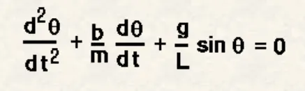
In the above equation,

g = gravity in m/s2,

L = length of the pendulum in m,

m = mass of the ball in kg,

b=damping coefficient.

Now to solve the above-mentioned 2nd order ODE, we need to simplify it to a 1st order ODE by assuming certain values and solving.

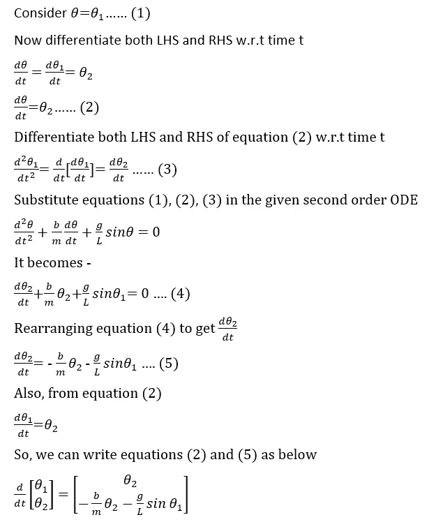
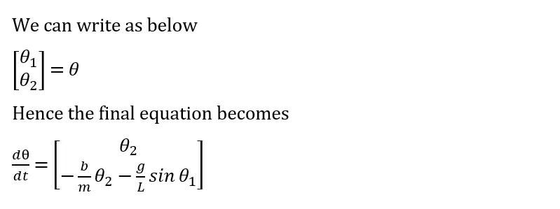
This above equation can be used as a solution array to solve the ODE using the ode45 syntax.

ode45 is a function in MATLAB that solves ordinary or partial differential equations using numerical method. The numerical method in question here is the 4th order Range Kutta method.

The function ode45 takes 3 inputs. The 3 inputs are the function to be integrated, the time span and the initial conditions. The function would be one like shown in the above equation. The time span would be the integration limits. This can be provided as a vector of 2 values, the initial and final time or with a spacing using the linspace function. The solver will choose a step size that is most suitable for the solution to obtain the solution in the most optimal time as possible. The initial condition would be the value of the function at t-0 seconds.

The function can be provided in the form of an anonymous function.

[t,results]=ode45(@(x)x^2,t_span,y0)

Here, we are saying that we don't know the value of x and x is an input to the anonymous function that we have defined here. This is equivalent to defining a function that takes the input of x and gives the output of x^2.

The function can also be defined as a separate function. This function must take at least 2 inputs, which should be t and y, apart from other arguments, where t would be the current time and y would be the value of the function at the previous time step.

Assuming we have a function ode, the function must be defined as,

function[outputs]=ode(t,y,args)

where args refer to any other arguments that the function may take.

This function must then be input to ode45 as

[t,results]=ode45(@(t,y)ode(t,y,args),tspan,y0)

This is necessary to tell the function which arguments of the function are to be found by the solver. Any ODE to be integrated by ode45 must be provided as a set of first order ODEs.

For animation of the simulation of pendulum motion, we need to plot coordinates of angular displacement i.e, the solution of the ODE. Consider the diagram shown below -

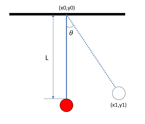
Coordinates (x0,y0) and (x1,y1) can be represented as follows from the diagram given below -

x0 = 0; y0 = 0

x1 = L*sin(THETA); y1 = -(L*cos(THETA))

L - Length of the pendulum; THETA - The angular displacement of the pendulum wrt time (solution of the ODE)

Using the above theory and solution, we can write a program to find the solution of a 2nd order ODE of the pendulum i.e., angular displacement and angular velocity at that particular time span.

PROGRAM -

%To Write a program in MATLAB that will simulate the pendulum motion.
%We need to use the given inputs and initial conditions.

close all
clear all
clc

%Inputs as provided
L=1;
m=1;
b=0.05;
g=9.81;

%Initial conditions, angular displacement=0; angular velocity=3
theta_0=[0;3];

%time points, time between 0-20 seconds 
t_span = linspace(0,20,500);

%Using ODE45 syntax to solve the ODE
%ode45 is the syntax used for solving an ODE. 
%@(t,theta) defines that the ODE is a function of t and theta
%pendulum_func is a function which is called here to solve the ODE
%t_span is the time interval needed for the integration of the ODE
%theta_0 defines the intial conditions of the pendulum

[t,results]=ode45(@(t,theta)pendulum_func(t,theta,L,m,b,g),t_span,theta_0);

%To plot the solutions i.e., angular displacements and angular velocities
%w.r.t time

figure(1)
plot(t,results(:,1))
hold on
plot(t,results(:,2))
xlabel('Time')
ylabel('Plot')

%To substitute the values of angular displacements into a more simpler
%variable 
displacement=results(:,1);

%To use the nested for loops to plot the animation of the pendulum motion 
%To capture frames and make a movie through MATLAB

ct=1;
for i=1:length(displacement)
   
   THETA = displacement(i);
        
        %To set the coordinates required to plot the angular displacement
        %of the pendulum at that particular time point
        
        %Assume length of the pendulum to be 1 m
        L=1;
        
        %The coordinates of the pendulum position is noted below
        x0=0;
        y0=0;
        
        x1= L*sin(THETA);
        y1= -(L*cos(THETA));
        
        figure(2)
        plot([x0,x1],[y0,y1],'linewidth',3)
        hold on
        plot(x1,y1,'o','MarkerSize',15,'MarkerEdgeColor','r','MarkerFaceColor','r') 
        hold off
        axis([-1 1 -1.1 0])
        pause(0.003)
  
        %To save all the images being plotted in the variable M
        M(ct)=getframe(gcf);  
        ct=ct+1;
        
end
    
%To make a movie/video of the simulation of the motion of pendulum
movie(M);

%To create a video file of the particular name and file 
videofile=VideoWriter('pendulum_motion_simulation','Uncompressed AVI');

%To open the video file created above and write all the frames that has
%been saved from the for loop
open(videofile)
writeVideo(videofile,M)
close(videofile)

The function which is being called in the program is written based on the theory explained above.

%To write a program as a function to be called for solving the ODE

function [dtheta_dt]=pendulum_func(t,theta,L,m,b,g)

%The explanation for the breakdown of a 2nd order ODE is given above 
%The same procedure is being followed here in this program

theta1=theta(1);
theta2=theta(2);

dtheta1_dt = theta2;
dtheta2_dt = -(b/m)*theta2-(g/L)*sin(theta1);

%Solutions are represented in the form of a column vector of the above
%values 
dtheta_dt = [dtheta1_dt;dtheta2_dt];

end

ERRORS FACED DURING EXECUTION -

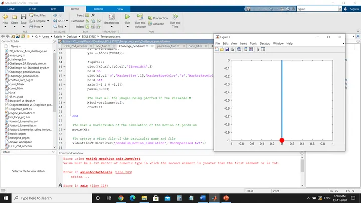
1. Error in line 69 - Value must be 1x2 vector of numeric type in which the second element is greater than the first element or is Inf.

Correction - axis([-1 1 0 -1.1]) -----> axis([-1 1 -1.1 0])

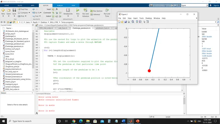
2. Error using movie, Movie contains uninitialised frames. This was because the counter variable was initialised with the number 2 (ct=2).

Correction - line 46, ct=2 -------> ct=1

RESULTS -

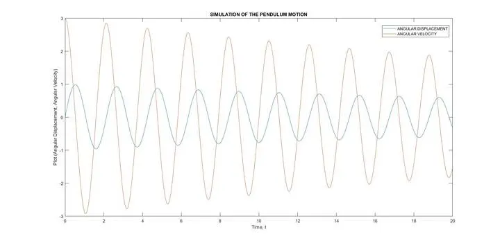
1. The plot representing the simulation of the pendulum motion is attached below (Simulation_of_pendulum_motion)

2. The link for the animation video of the simulation of the pendulum motion is attached below (pendulum_motion_simulation)

https://drive.google.com/file/d/1OpAyekGWkXJStwlSA-iau-gcfCffmvSK/view?usp=sharing