FITTING A LINEAR AND CUBIC POLYNOMIAL FOR THE PROVIDED Cp DATA USING CONVENTIONAL METHOD AND SPLIT-WISE METHOD WITH VALIDATION OF THE GOODNESS OF THE CURVE

AIM -

1. To write a code to fit a linear and cubic polynomial for the Cp data. Plot the linear and cubic fit curves along with the raw data points.
2. To write a code to show the split-wise method.
3. Explain the parameters used to measure the fitness characteristics for both the curves.

Based on the research done, answer the following -

1. How to make a curve fit perfectly?
2. How to get the best fit?
3. What could be done to improve the cubic fit?

THEORY -

Curve fitting is the way we model or represent a data spread by assigning the best fit curve along with the entire range. Ideally, it will capture the trend in the data and allow us to make predictions of how the data series will behave in the future.

There are different ways to determine what is the 'best' match. If the curve has to go through the data points, we have interpolation. In least-squares curve fitting, the sum of the squares of the residuals (the difference between the data value and the value predicted by the curve) is minimized. In weighted least squares, each data point is assigned a weight that indicates how much the data point influences the parameters.

Types of curve fitting include:

• Interpolation, where you discover a function that is an exact fit to the data points. Since this assumes no measurement error, it has limited applicability to real-life scenarios.
• Smoothing/Curve fitting is when we find a function that is an approximate fit to the data points, but we give room for error and we allow our actual points to be near, but not necessarily on the line; given the error is minimized overall.

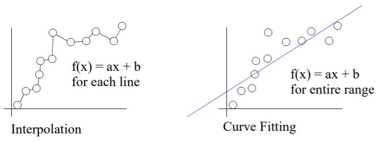
Also, there are different types of curve fitting/smoothing -

1. Linear curve fitting (Linear Regression)

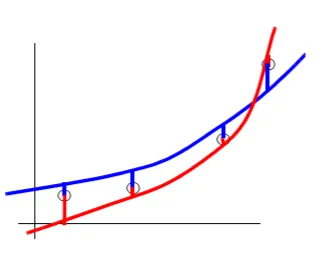
Consider the general form of a straight line, f(x) = ax + b. We need to pick the coefficients a and b that best fit the line to the data. The one line that provides a minimum error is then the best straight line which defines the equation.

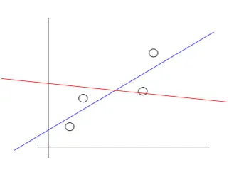
In the above example, the blue line is the best fit for the data as the error is minimum when compared to the red line.

To find the coefficients a and b, we need to quantify the error in the curve fit first. To get the positive value of the error, we need to square it. (Data points are above or below the line). Denote the data values as (x,y) and denote the points on the fitted line as (x,f(x)).

The best line has minimum errors between line and data points. This is called the least-squares method since we minimize the square of the error.

Using the above theory, the error equation is as follows -

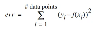
As f(x) = ax + b, substituting this in the above equation we get,

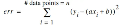
Now to find the minimum of a function 1. Derivative describes a slope 2. Slope = 0 is a minimum.

Take the derivative of the error with respect to a and b, set each to zero.

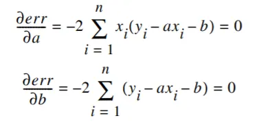
Solve for a and b and re-write these two equations

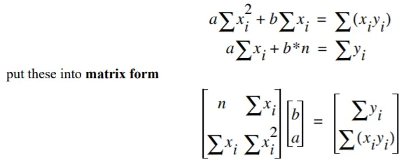
Using the Gaussian elimination find out the coefficients a and b.

2. Polynomial Curve Fitting (Polynomial Regression) -

Consider the general form for a polynomial of order j

Just as the case for linear regression, we pick the coefficients that best fit the curve to the data. So, now we quantify the error for these second-order curves and pick the curve with the minimum total error.

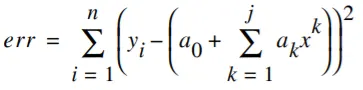
The general expression for any error using the least-squares method is -

Substituting the f(x) value to the above equation -

To minimize the error, we take the derivative

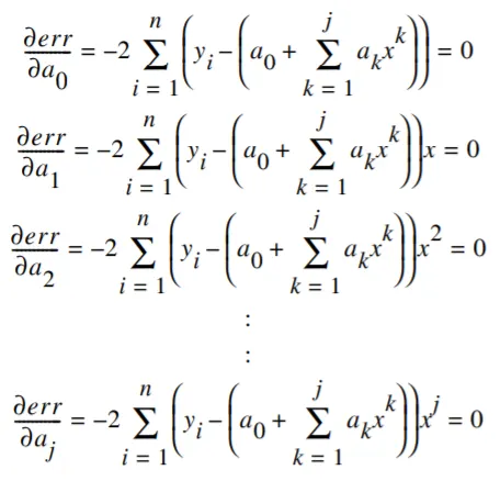
Now, we re-write these equations and put it into matrix form

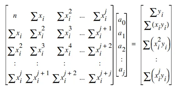
Using the Gaussian elimination method, we find the coefficients of the polynomial equation.

The above theory was about linear curve fitting, there are also different types of non-linear curve fitting.

1. Exponential curve fitting

2. Logistic curve fitting

We won't be going in-depth about these two as it is beyond the scope of this project.

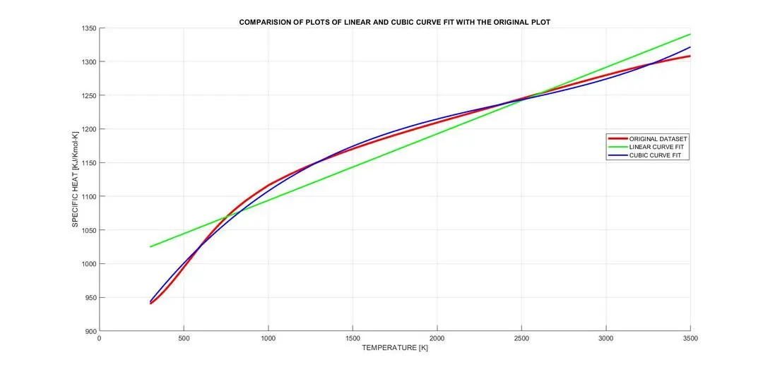
In the program, we have plotted the linear and cubic polynomial for the Cp data along with its original plot from the raw dataset. Along with this, we have also evaluated the goodness of the fit and its error criteria.

We have evaluated by calculating the values of the following parameters -

1. The sum of squares due to error (SSE)

2. R-square

3. Adjusted R-square

4. Root mean squared error (RMSE)

Each of them has been explained below -

1. SSE method -

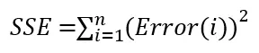
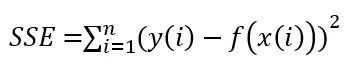
The method is known as the Least squares method and is a common technique for a polynomial function. This statistic measures the total deviation of the response values from the fit to the response values. It is also called the summed squares of residuals and is usually labeled SSE. A value closer to 0 indicates a better fit.

From the above explanation, we know,

f(x) being the function representing the data and y(i) being the raw data.

2. R-square -

This quantity measures how successful the fit is in explaining the variation of the data. It is the square of the correlation between the response values and the predicted response values.

The higher the value of R-square the better the fit, the lower the value the poorer the fit.

The values range from 0-1. 0 being the worst fit for the data set, 1 being the best fit for the data set. The value of the R-square can be calculated using the following formula

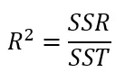
SSR - the sum of squares of the regression, which is basically the square of the difference between the value of the fitting function at a given point and the arithmetic mean of the data set.

If y=f(x) is the fit curve then the SSR is defined as follows -

Similarly, SSE will be taken from above,

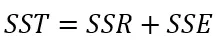
Now the term SST is nothing but the sum of SSE and SSR,

3. Adjusted R-square -

Adjusted R-square is a normalizing variation of R-square which neglects the variation of R-Square due to insignificant independent variables.

It considers the variables which actually contribute to the output of the system in a drastic way.

R-sqaure_adjusted is formulated as shown below -

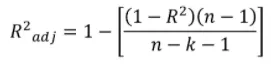
where,

n - the number of data points

k - the number of independent variables

There are 2 possibilities - 1. The newly added independent variable is significant 2. The newly added independent variable is insignificant

4. RMSE (Root Mean Squared Error) -

This is also known as a fit standard error and the standard error of the regression. It is an estimate of the standard deviation of the random component in the data and is defined as,

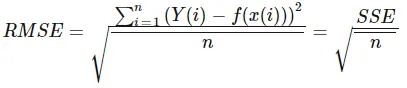
where n is the total number of data points available.

Using these four quantities MATLAB effectively deduces the goodness of fit, if R-square is greater than 0.95 the fit is assumed to be good.

The code to fit a linear and cubic polynomial for the Cp data is as follows -

%To plot the code to fit a linear and cubic polynomial for the Cp data and
%To plot a comparison plot of both these curves with the original curve

clear all
close all
clc

%Preparing Data of Temperature, T and Specific heat, cp
DATA = load('data');
temperature = DATA(:,1);
cp = DATA(:,2);

%To plot a linear fit curve along the raw data points
%Consider the linear equation, cp = A*T + B
linear_coeffs = polyfit(temperature,cp,1);
cp_linear = polyval(linear_coeffs,temperature);
 
%To plot a cubic fit curve along the raw data points
%Consider the 3rd degree polynomial equation, cp = A*T^3 + B*T^2 + C*T + D
cubic_coeffs = polyfit(temperature,cp,3);
cp_cubic = polyval(cubic_coeffs,temperature);

%Comparing the linear and cubic curve fit with the orignal plot
figure(1)
hold on
plot(temperature,cp,'linewidth',3,'color','r')
plot(temperature,cp_linear,'linewidth',2,'color','g')
plot(temperature,cp_cubic,'linewidth',2,'color','b')
xlabel('TEMPERATURE [K]')
ylabel('SPECIFIC HEAT [KJ/Kmol-K]')
grid on
legend('ORIGINAL DATASET','LINEAR CURVE FIT','CUBIC CURVE FIT')
title('COMPARISION OF PLOTS OF LINEAR AND CUBIC CURVE FIT WITH THE ORIGINAL PLOT')

%To evaluate the fitness characteristics of both curves
%We will be adopting the sum of squares due to errors(SSE) method
% Error = sum of |y(i)-f(x(i))|
% SSE = sum(Error(i)^2) = sum(|y(i)-f(x(i))|.^2)

% To find SSE of the linear fit curve
error_linear = cp-cp_linear;
SSE_linear = sum(error_linear.^2)

% To find SSE of the linear fit curve
error_cubic = cp-cp_cubic;
SSE_cubic = sum(error_cubic.^2)

%To find the R_square values of both the curves 
% R_square = SSR/SST
% SSR = sum((cp_linear-MEAN).^2)
% SST = SSR+SSE
% SSE has been calculated for both the curves above

MEAN = mean(cp);

%To find R_square of the linear curve
SSR_linear = sum((cp_linear-MEAN).^2);
SST_linear = SSR_linear+SSE_linear;
R_square_linear = SSR_linear./SST_linear

%To find R_square of the cubic curve
SSR_cubic = sum((cp_cubic-MEAN).^2);
SST_cubic = SSR_cubic+SSE_cubic;
R_square_cubic = SSR_cubic./SST_cubic

%To find adjusted R_square for both the curves
%R_square_adj = 1-((1-R_square)*(n-1)/(n-k-1))
% n is the number of datapoints
% k is the number of independent variables 

n = 3200;
k = 1;

%The value of R_square_adj of the linear curve 
R_square_adj_linear = 1-((1-R_square_linear)*(n-1)/(n-k-1))

%The value of R_square adj of the cubic curve
R_square_adj_cubic = 1-((1-R_square_cubic)*(n-1)/(n-k-1))

%To find the RMSE values of both the curves
% RMSE = sqrt(SSE/n)
% SSE being the sum of the squares due to errors calculated above

%The RMSE value of the linear curve
RMSE_linear = sqrt(SSE_linear/n)

%The RMSE value of the cubic curve
RMSE_cubic = sqrt(SSE_cubic/n)

Results for the above program are shown below -

1. Plot of the linear and cubic curve fit with its comparison with the original plot is shown below -

2. The values of the parameters which evaluates the goodness of the fit is tabulated as below -

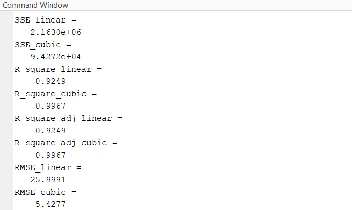
PARAMETERS	LINEAR	CUBIC
SSE (sum of squared errors)	2.1630e+06	9.4272e+04
R-square	0.9249	0.9967
Adjusted R-square	0.9249	0.9967
RMSE	25.9991	5.4277

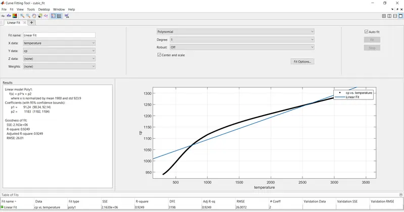
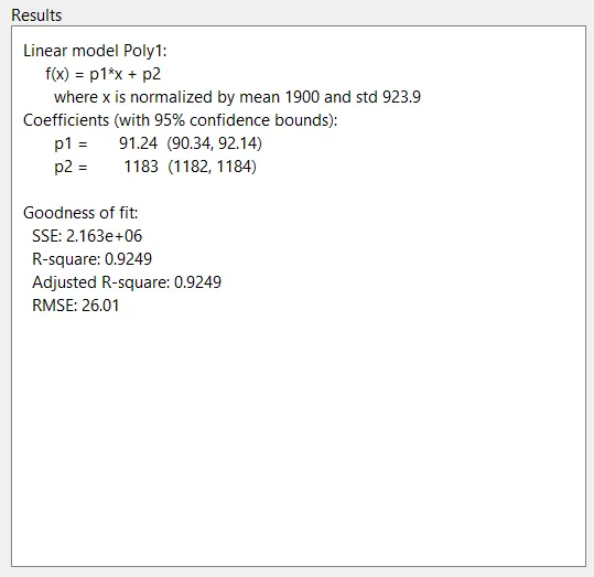
3. Comparision of the above results with the results obtained from the curve fit toolbox -

a) Linear fit -

b) Cubic fit -

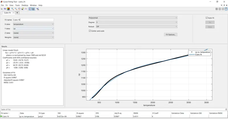
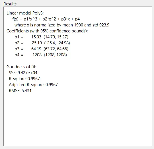
Comparing the values of parameters evaluating the goodness of fit obtained in the curve fit toolbox with the results mentioned in the table above, we can see that the values are equal or close to each other. This shows the correctness of the program and also confirms the fitness of the curve.

The code to find the best fit for the curve using the split-wise method is shown below -

%To write a code to show the split-wise method and compare the plots with
%the original plot 

clear all
close all
clc

%Preparing the data
DATA = load('data');
temperature = DATA(:,1);
cp = DATA(:,2);

%To obtain a more accurate curve fitting for the available dataset
%We split up the data into multiple linear equations and then plot the data
%separately.
%We then compare all the multiple plots together with the original plot 

%Preparing data for each of the split equations 
%To plot a linear curve for the first equation 
temperature_1 = temperature(1:640);
cp_1 = cp(1:640);
%Consider cp1 = A*T1 + B
coeff_1 = polyfit(temperature_1, cp_1,1);
predicted_cp_1=polyval(coeff_1,temperature_1);

%To plot a linear curve for the second equation
temperature_2 = temperature(641:1280);
cp_2 = cp(641:1280);
%Consider cp2 = C*T2 + D
coeff_2 = polyfit(temperature_2, cp_2,1);
predicted_cp_2=polyval(coeff_2,temperature_2);

%To plot a linear curve for the third equation
temperature_3 = temperature(1281:1920);
cp_3 = cp(1281:1920);
%Consider cp3 = E*T3 + F
coeff_3 = polyfit(temperature_3, cp_3,1);
predicted_cp_3=polyval(coeff_3,temperature_3);

%To plot a linear curve for the fourth equation
temperature_4 = temperature(1921:2560);
cp_4 = cp(1921:2560);
%Consider cp4 = G*T4 + H
coeff_4 = polyfit(temperature_4, cp_4,1);
predicted_cp_4=polyval(coeff_4,temperature_4);

%To plot a linear curve for the fifth equation
temperature_5 = temperature(2561:3200);
cp_5 = cp(2561:3200);
%Consider cp5 = I*T2 + J
coeff_5 = polyfit(temperature_5, cp_5,1);
predicted_cp_5=polyval(coeff_5,temperature_5);

%Comparing the original plot with the plots of each of the equations 
figure(1)
hold on
plot(temperature,cp,'linewidth',5,'color','r')
plot(temperature_1,cp_1,'linewidth',2,'color','g')
plot(temperature_2,cp_2,'linewidth',2,'color','y')
plot(temperature_3,cp_3,'linewidth',2,'color','b')
plot(temperature_4,cp_4,'linewidth',2,'color','white')
plot(temperature_5,cp_5,'linewidth',2,'color','black')
xlabel('TEMPERATURE [K]')
ylabel('SPECIFIC HEAT [KJ/Kmol-K]')
legend('ORIGINAL DATASET','CURVE FIT OF EQN1','CURVE FIT OF EQN2','CURVE FIT OF EQN3','CURVE FIT OF EQN4','CURVE FIT OF EQN5')
title('COMPARISION OF PLOTS OF ALL SPLIT EQUATIONS WITH THE ORIGINAL PLOT')
grid on

%To evaluate the fitness characteristics of all the linear fit curves
%We will be adopting the sum of squares due to errors(SSE) method
% Error = sum of |y(i)-f(x(i))|
% SSE = sum(Error(i)^2) = sum(|y(i)-f(x(i))|.^2)

% To find SSE of the 1st linear fit curve
error_1 = cp_1-predicted_cp_1;
SSE_1 = sum(error_1.^2)

% To find SSE of the 2nd linear fit curve
error_2 = cp_2-predicted_cp_2;
SSE_2 = sum(error_2.^2)

% To find SSE of the 3rd linear fit curve
error_3 = cp_3-predicted_cp_3;
SSE_3 = sum(error_3.^2)

% To find SSE of the 4th linear fit curve
error_4 = cp_4-predicted_cp_4;
SSE_4 = sum(error_4.^2)

% To find SSE of the 5th linear fit curve
error_5 = cp_5-predicted_cp_5;
SSE_5 = sum(error_5.^2)

%To find the R_square values of both the curves 
% R_square = SSR/SST
% SSR = sum((cp_linear-MEAN).^2)
% SST = SSR+SSE
% SSE has been calculated for both the curves above

%To find R_square of the 1st linear curve
MEAN_1 = mean(cp_1);
SSR_1 = sum((cp_1-MEAN_1).^2);
SST_1 = SSR_1+SSE_1;
R_square_1 = SSR_1./SST_1

%To find R_square of the 2nd linear curve
MEAN_2 = mean(cp_2);
SSR_2 = sum((cp_2-MEAN_2).^2);
SST_2 = SSR_2+SSE_2;
R_square_2 = SSR_2./SST_2

%To find R_square of the 3rd linear curve
MEAN_3 = mean(cp_3);
SSR_3 = sum((cp_3-MEAN_3).^2);
SST_3 = SSR_3+SSE_3;
R_square_3 = SSR_3./SST_3

%To find R_square of the 4th linear curve
MEAN_4 = mean(cp_4);
SSR_4 = sum((cp_4-MEAN_4).^2);
SST_4 = SSR_4+SSE_4;
R_square_4 = SSR_4./SST_4

%To find R_square of the 5th linear curve
MEAN_5 = mean(cp_5);
SSR_5 = sum((cp_5-MEAN_5).^2);
SST_5 = SSR_5+SSE_5;
R_square_5 = SSR_5./SST_5

%To find adjusted R_square for both the curves
%R_square_adj = 1-((1-R_square)*(n-1)/(n-k-1))
% n is the number of datapoints
% k is the number of independent variables 

n = 640;
k = 1;

%The value of R_square_adj of the 1st linear curve 
R_square_adj_1 = 1-((1-R_square_1)*(n-1)/(n-k-1))

%The value of R_square_adj of the 2nd linear curve 
R_square_adj_2 = 1-((1-R_square_2)*(n-1)/(n-k-1))

%The value of R_square_adj of the 3rd linear curve 
R_square_adj_3 = 1-((1-R_square_3)*(n-1)/(n-k-1))

%The value of R_square_adj of the 4th linear curve 
R_square_adj_4 = 1-((1-R_square_4)*(n-1)/(n-k-1))

%The value of R_square_adj of the 5th linear curve 
R_square_adj_5 = 1-((1-R_square_5)*(n-1)/(n-k-1))

%To find the RMSE values of both the curves
% RMSE = sqrt(SSE/n)
% SSE being the sum of the squares due to errors calculated above

%The RMSE value of the 1st linear curve
RMSE_1 = sqrt(SSE_1/n)

%The RMSE value of the 2nd linear curve
RMSE_2 = sqrt(SSE_2/n)

%The RMSE value of the 3rd linear curve
RMSE_3 = sqrt(SSE_3/n)

%The RMSE value of the 4th linear curve
RMSE_4 = sqrt(SSE_4/n)

%The RMSE value of the 5th linear curve
RMSE_5 = sqrt(SSE_5/n)

In this code, the temperature and cp have been split into 5 different linear equations. So the total of 3200 values will be split into 640 each.

Each of these equations will be solved using the polyfit and polyval command. The values obtained will be used to plot the graph and then be compared with the original plot.

Results for the above program are shown below -

1. The curve fit obtained using the split-wise method and its comparison with the original plot is as shown below -

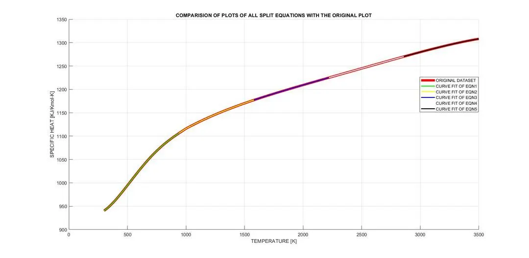
2. The values of the parameters which evaluates the goodness of the fit is tabulated as below -

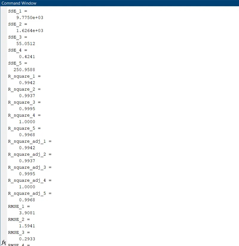
PARAMETERS	1ST LINEAR EQUATION	2ND LINEAR EQUATION	3RD LINEAR EQUATION	4TH LINEAR EQUATION	5TH LINEAR EQUATION
SSE (sum of squared errors)	9.7750e+03	1.6264e+03	55.0512	0.4241	250.9588
R-square	0.9942	0.9937	0.9995	1.0000	0.9968
Adjusted R-square	0.9942	0.9937	0.9995	1.0000	0.9968
RMSE	3.9081	1.5941	0.2933	0.0257	0.6262

Based on the study, the questions will be answered

1. How to make a curve fit perfectly?

The perfect fit is the curve with a value of R-square close to 1 which means the curve which fits the original dataset with minimum error. The perfect fit can always be the best fit but the best fit cannot always be the perfect fit. To check the goodness of the fit, we evaluate certain parameters and we can say that any curve with the value of R-square greater than 0.95 is the curve that will fit the dataset perfectly.

2. How to get the best fit?

To get the best fit, we first evaluate the parameters for characteristic curve fitting. The values of SSE which is obtained by the least-squares method which is a common technique used. We can also determine the value of R-square or the adjusted R-square and also the value of RMSE value. The 'best' fit can be determined by evaluating the values of the above-mentioned parameters. To improve the current fit, we can increase the order of the polynomial or also use the split-wise method which will minimize the errors.

3. What could be done to improve the cubic fit?

The problem with the cubic fit is that the equation is very unstable and MATLAB shows us the warning in the command window. The meaning of the instability is that a slight variation in the variable would result in a large variation in the output. So to avoid this we can use the split-wise method, here we split the dataset into multiple cubic equations or linear equations and solve each of these separately and plot them. This also leads to minimizing the errors and would act as the best fit for the given dataset.

CONCLUSION -

In this project, we find the linear and cubic fit for the Cp data provided and also compare it with the original plot. We evaluate the fitness of the curve by calculating the SSE, R-Square, Adjusted R-square, and RMSE values for both the curves. We also find the best fit for the given Cp data using the split-wise method and we obtained the goodness parameters for each of those equations too. All the results and plots are attached in the results section.

REFERENCES -

1. https://skill-lync.com/projects/Curve-Fitting-and-criterion-to-choose-best-fit-41860

2. https://skill-lync.com/knowledgebase/the-basic-concept-of-curve-fit

3. https://in.mathworks.com/help/curvefit/evaluate-a-curve-fit.html

4. https://www.extremeoptimization.com/Documentation/Mathematics/Curve-Fitting/Default.aspx

5. https://statisticsbyjim.com/regression/curve-fitting-linear-nonlinear-regression/

6. https://nptel.ac.in/content/storage2/courses/104101002/downloads/lecture-notes/module1/chapter4.pdf