Challenge

OPTIMIZATION OF A STALAGMITE FUNCTION AND TO FIND ITS GLOBAL MAXIMA DOING A STATISTICAL BEHAVIOR STUDY OF THE FUNCTION

RRajath Ulvekar26 Nov 2020

AIM -

1. To write a code in MATLAB to optimize the stalagmite function and find the global maxima of the function, make sure that the code gives the same output, even if it is made to run several times. Plot graphs for all 3 studies and F maximum vs no. of iterations. Title and axes labels are a must, legends could be shown if necessary

2. To clearly explain the concept of genetic algorithm and also explain the syntax for ga in MATLAB in your report.

THEORY -

Before looking into what the Genetic algorithm is, we need to know what is optimization.

An optimization algorithm is a procedure that is executed iteratively by comparing various solutions until an optimum or a satisfactory solution is found. In the optimization of a design, the design objective could be simply to minimize the cost of production or to maximize the efficiency of production. There are 2 distinct types of optimization algorithms widely used today.

Deterministic Algorithms - They use specific rules for moving one solution to another. These algorithms are in use to suit some times and have been successfully applied for many engineering design problems.
Stochastic Algorithms - The stochastic algorithms are in nature with probabilistic translation rules. These are gaining popularity due to certain properties that deterministic algorithms do not have.

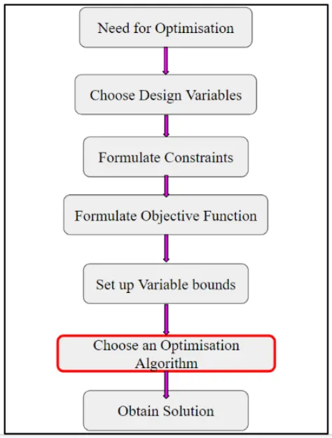
The below picture depicts the procedure followed by any optimization process.

A genetic algorithm (GA) is a method for solving both constrained and unconstrained optimization problems based on a natural selection process that mimics biological evolution. The algorithm repeatedly modifies a population of individual solutions. At each step, the genetic algorithm randomly selects individuals from the current population and uses them as parents to produce the children for the next generation. Over successive generations, the population evolves toward an optimal solution.

We can apply the genetic algorithm to solve problems that are not well suited for standard optimization algorithms, including problems in which the objective function is discontinuous, nondifferentiable, stochastic, or highly nonlinear.

A brief explanation of how the genetic algorithm works -

1. The algorithm begins by creating a random initial population.

2. The algorithm then creates a sequence of new populations. At each step, the algorithm uses the individuals in the current generation to create the next population. To create a new population, the algorithm performs the following steps.

a. Scores each member of the current population by computing its fitness value. These values are called raw fitness scores.

b. Scales the raw fitness scores to convert them into a more usable range of values. These scaled values are called expectation values.

c. Selects members, called parents, based on their expectation values.

d. Some of the individuals in the current population that have lower fitness are chosen as elite. These elite individuals are passed to the next population.

e. Produces children from selected parents. Children are produced either by making random changes to a single parent or by combining the vector entries of a pair of parents

f. Replaces the current population with the children to form the next generation.

3. The algorithm stops when one of the stopping criteria is met.

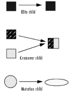
The genetic algorithm uses the individuals in the current generation to create the children that make up the next generation. Besides elite children, which correspond to the individuals in the current generation with the best fitness values, the algorithm creates

Crossover children by selecting vector entries, or genes, from a pair of individuals in the current generation and combines them to form a child. The algorithm creates crossover children by combining pairs of parents in the current population. At each coordinate of the child vector, the default crossover function randomly selects an entry, or gene, at the same coordinate from one of the two parents and assigns it to the child. For problems with linear constraints, the default crossover function creates the child as a random weighted average of the parents.
Mutation children by applying random changes to a single individual in the current generation to create a child. The algorithm creates mutation children by randomly changing the genes of individual parents. By default, for unconstrained problems, the algorithm adds a random vector from a Gaussian distribution to the parent. For bounded or linearly constrained problems, the child remains feasible.

Both processes are essential to the genetic algorithm. Crossover enables the algorithm to extract the best genes from different individuals and recombine them into potentially superior children. Mutation adds to the diversity of a population and thereby increases the likelihood that the algorithm will generate individuals with better fitness values.

The following schematic diagram illustrates the three types of children -

The termination condition of a genetic algorithm is important in determining when a GA run will end. It has been observed that, initially, the GA progresses very fast with better solutions coming in every few iterations, but this tends to saturate in the later stages where the improvements are very small. We usually want a termination condition such that our solution is close to the optimal at the end of the run.

Stopping conditions for the algorithm -

The genetic algorithm uses the following options to determine when to stop.

MaxGenerations — The algorithm stops when the number of generations reaches MaxGenerations.
MaxTime — The algorithm stops after running for an amount of time in seconds equal to MaxTime.
FitnessLimit — The algorithm stops when the value of the fitness function for the best point in the current population is less than or equal to FitnessLimit.
MaxStallGenerations — The algorithm stops when the average relative change in the fitness function value over MaxStallGenerations is less than Function tolerance.
MaxStallTime — The algorithm stops if there is no improvement in the objective function during an interval of time in seconds equal to MaxStallTime.
FunctionTolerance — The algorithm runs until the average relative change in the fitness function value over MaxStallGenerations is less than Function tolerance.
ConstraintTolerance — The ConstraintTolerance is not used as a stopping criterion. It is used to determine the feasibility with respect to nonlinear constraints. Also, max(sqrt(eps),ConstraintTolerance) determines feasibility with respect to linear constraints.

The algorithm stops as soon as any one of these conditions is met.

Advantages of GAs

GAs have various advantages that have made them immensely popular. These include −

Does not require any derivative information (which may not be available for many real-world problems).
Is faster and more efficient as compared to the traditional methods.
Has very good parallel capabilities.
Optimizes both continuous and discrete functions and also multi-objective problems.
Provides a list of “good” solutions and not just a single solution.
Always gets an answer to the problem, which gets better over time.
Useful when the search space is huge, and there are a large number of parameters involved.

Limitations of GAs

Like any technique, GAs also suffer from a few limitations. These include −

GAs are not suited for all problems, especially problems that are simple and for which derivative information is available.
The fitness value is calculated repeatedly which might be computationally expensive for some problems.
Being stochastic, there are no guarantees on the optimality or the quality of the solution.
If not implemented properly, the GA may not converge to the optimal solution.

The syntax used in the program for the genetic algorithm is a built-in command in MATLAB and is explained below

x=ga(fun,nvars)

x=ga(fun,nvars,A,b)

x=ga(fun,nvars,A,b,Aeq,beq)

x=ga(fun,nvars,A,b,Aeq,beq,lb,ub)

x=ga(fun,nvars,A,b,Aeq,beq,lb,ub,nonlcon)

x=ga(fun,nvars,A,b,Aeq,beq,lb,ub,nonlcon,options)

ga - the in-built command in MATLAB called while optimizing the function using the genetic algorithm.

fun - the function to be optimized

nvars - the number of variables in the function

A and b - are the linear inequality constraints of the function

Aeq and beq - are the equality constraints of the function

lb and ub - are the lower bounds and upper bounds of the solution required (the range in which the solution is required)

nonlcon - are the non-linear constraints of the function

options - the options where we define the other factors such as population size is defined

The fitness function to be solved is explained below -

The fitness function takes the solution as input and produces the suitability of the solution as the output. This evaluates how close the solution is to the optimal solution of the desired problem. We will be performing the genetic algorithm optimization for a stalagmite function to find its minima. The stalagmite function has two inputs x and y as shown in the below figure -

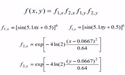
Now, what the fitness function will do is, it will find the value of 'f' by varying the sign as well as the value of the input arguments x and y and find the f value that should be as a minimum as possible. Now it will compare this fitness value with the optimized value of 'f' for every iteration and check how good the fit is. When we run this stalagmite function in MATLAB, we get a plot as shown below.

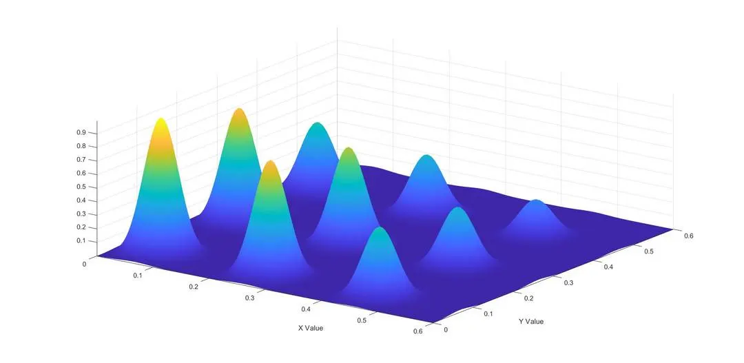
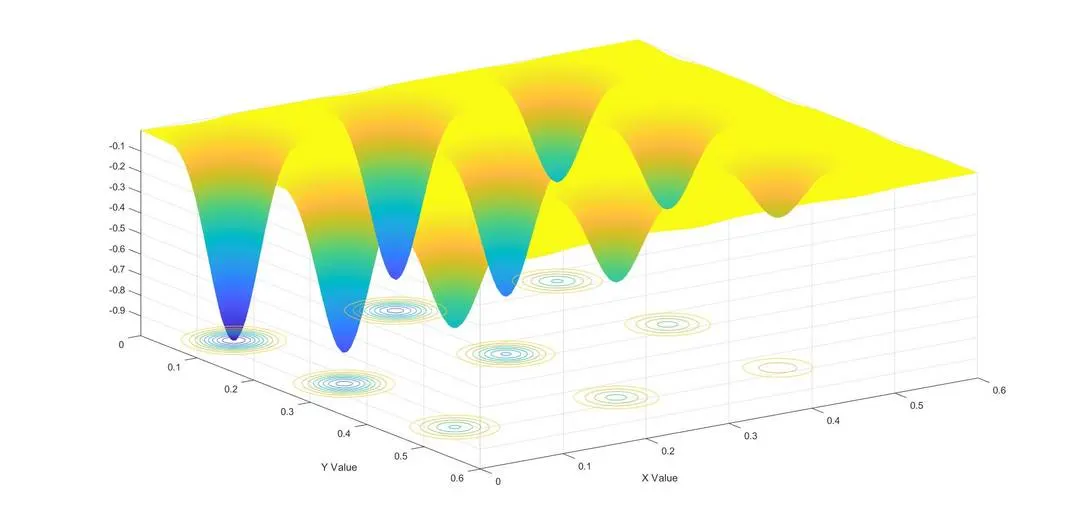
This plot shows that there are many local maxima and to find the global maxima we need to narrow down our search space to the highest peak in the above plot. But our ga command in MATLAB finds the most minimum value of the function, so to find our global maxima, we need to invert the given stalagmite function i.e., add a negative sign to our function. The ga command when solves the function, will be getting the minimum value which nothing but our global maxima with a negative sign. The inverted stalagmite function when run is shown below.

The code is written as follows -

%To write a code in MATLAB to optimize the stalagmite function and find the
%global maxima of the function
%To plot all 3 studies and f maximums vs no of iterations

clear all
close all
clc

%Determine the search space for the function 
x=linspace(0,0.6,150);
y=linspace(0,0.6,150);

%Creating a 2-D mesh 
[xx,yy]=meshgrid(x,y);

%Evaluating the stalagmite function 
for i=1:length(xx)
    for j=1:length(yy)
        
        input_vector(1)=xx(i,j);
        input_vector(2)=yy(i,j);
        %The stalagmite function is written and explained in detail 
        %The program for the function has been attached below 
        f(i,j)=get_stalagmite(input_vector);
        
    end
end

%Setting the number of iterations for the GA
num_cases=50;

%Study - 1 - Statistical behaviour - with unbounded inputs
%We also will be evaluating the time taken to determine the study time for
%all cases using the tic and toc command 
tic
for i=1:num_cases
    %will be using the in-built ga command to solve the function 
    %the function and number of variables are mentioned as inputs are
    %unbound
    [inputs1,fopt1(i)]= ga(@get_stalagmite,2);
    xopt1(i)=inputs1(1);
    yopt1(i)=inputs1(2);
end
study1_time=toc

%To plot the results of study - 1
%Create subplots where the first plot will be of the 3-D surface and the
%second plot will be function minimum vs iterations 
figure(1)
subplot(2,1,1)
hold on
surfc(xx,yy,f)
shading interp
plot3(xopt1,yopt1,fopt1,'marker','o','markersize',5,'markerfacecolor','r')
title('Unbounded inputs')
subplot(2,1,2)
plot(fopt1)
xlabel('Iterations')
ylabel('Function minimum')

%Study - 2 - Statistical behaviour - with upper and lower bounds
%We also will be evaluating the time taken to determine the study time for
%all cases using the tic and toc command 
tic
for i=1:num_cases
    %will be using the in-built ga command to solve the function 
    %the function,number of variables and the lower bound and upper bound
    %of the input is specified 
    [inputs2,fopt2(i)]=ga(@get_stalagmite,2,[],[],[],[],[0;0],[0.6;0.6]);
    xopt2(i)=inputs2(1);
    yopt2(i)=inputs2(2);
end
study2_time=toc

%To plot the results of study - 2
%Create subplots where the first plot will be of the 3-D surface and the
%second plot will be function minimum vs iterations 
figure(2)
subplot(2,1,1)
hold on
surfc(xx,yy,f)
shading interp
plot3(xopt2,yopt2,fopt2,'marker','o','markersize',5,'markerfacecolor','r')
title('Bounded inputs')
subplot(2,1,2)
plot(fopt2)
xlabel('Iterations')
ylabel('Function minimum')

%Study - 3 - introducing population size
%We also will be evaluating the time taken to determine the study time for
%all cases using the tic and toc command 
%We will be using the optimoptions to set the population size for the
%current search space and set it to 200
options = optimoptions('ga');
options = optimoptions(options,'PopulationSize',200);

%We also will be evaluating the time taken to determine the study time for
%all cases using the tic and toc command 
tic
for i=1:num_cases
    %will be using the in-built ga command to solve the function 
    %the function, number of variables, the lower bound and upper bound
    %and the population size of the input is specified 
    [inputs3,fopt3(i)]=ga(@get_stalagmite,2,[],[],[],[],[0;0],[0.4;0.4],[],[],options)
    xopt3(i)=inputs3(1);
    yopt3(i)=inputs3(2);
end
study3_time=toc

%To plot the results of study - 3
%Create subplots where the first plot will be of the 3-D surface and the
%second plot will be function minimum vs iterations
figure(3)
subplot(2,1,1)
hold on
surfc(xx,yy,f)
shading interp
plot3(xopt3,yopt3,fopt3,'marker','o','markersize',5,'markerfacecolor','r')
title('Inputs after increasing GA iterations')
subplot(2,1,2)
plot(fopt3)
xlabel('Iterations')
ylabel('Function Minimum')

The function called get_stalagmite has been called in the above program to solve the given stalagmite function which has been explained above.

The code for the function is given below -

%To write a function code to solve the stalagmite function which has been
%explained above 
function [f]=get_stalagmite(input_vector)

%Substituting the input_vector in the x and y variables 
x=input_vector(1);
y=input_vector(2);

%To solve the stalagmite function 
f1_x=(sin(5.1*pi*x+0.5))^6;
f1_y=(sin(5.1*pi*y+0.5))^6;
f2_x=exp(-4*log(2)*(x-0.0667)^2/0.64);
f2_y=exp(-4*log(2)*(y-0.0667)^2/0.64);

%The negative sign is to make sure we get the maximum value of the function
%with a negative sign as ga always finds the minimum value of the function
[f]=-(f1_x*f2_x*f1_y*f2_y);

end

Once we run the above program we will be getting the plots and the global maxima of the function in all the 3 studies mentioned. They are explained in the below section.

ERRORS -

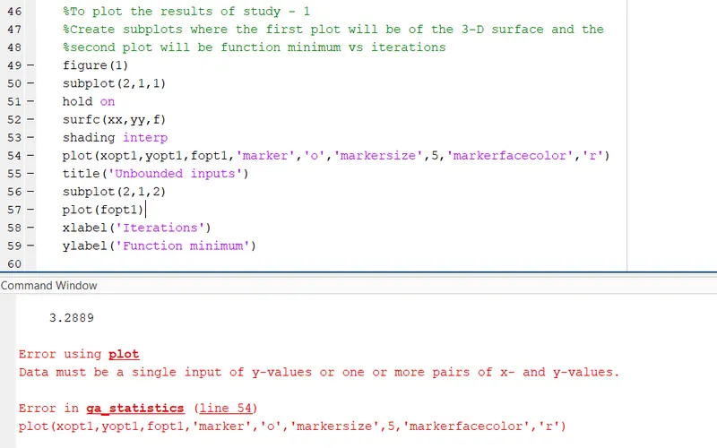
As we can see in the above image, the error was in using the plot command instead of the plot3 command. Once this was changed, the program didn't face any other errors.

RESULTS -

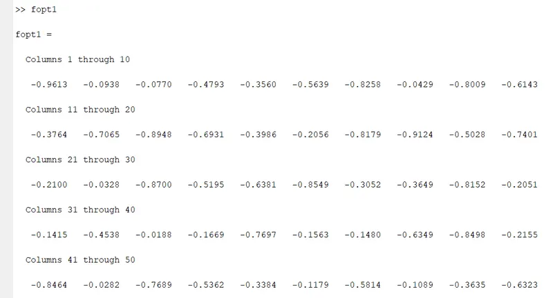
1. Study -1 - Statistical behavior of the function when the inputs are unbound. The results and plots when the inputs are not bounded by any limits, and no constraints are shown below. We can see that the function maximas vary beyond our search space and is varying from -1 to 0 for 50 iterations too many times. So, this result won't be acceptable as we are not able to find the global maxima within our search space.

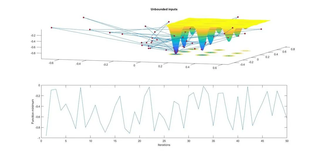
We can see from the below figure that the results vary a lot for the number of iterations set.

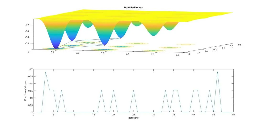
2. Study -2 - Statistical behavior of the function when the inputs are bounded. In this study, we have set a lower and upper bound for the inputs, 0-0.6. Hence the results obtained would be within the range provided with very less variations of the maximas for the set iterations. The result is acceptable with room for improvement.

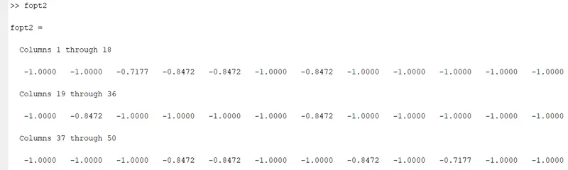
The fopt2 values (the function minimas) for study-2 has been shown below. We can see that the variation of the values has decreased when compared to study-1 results.

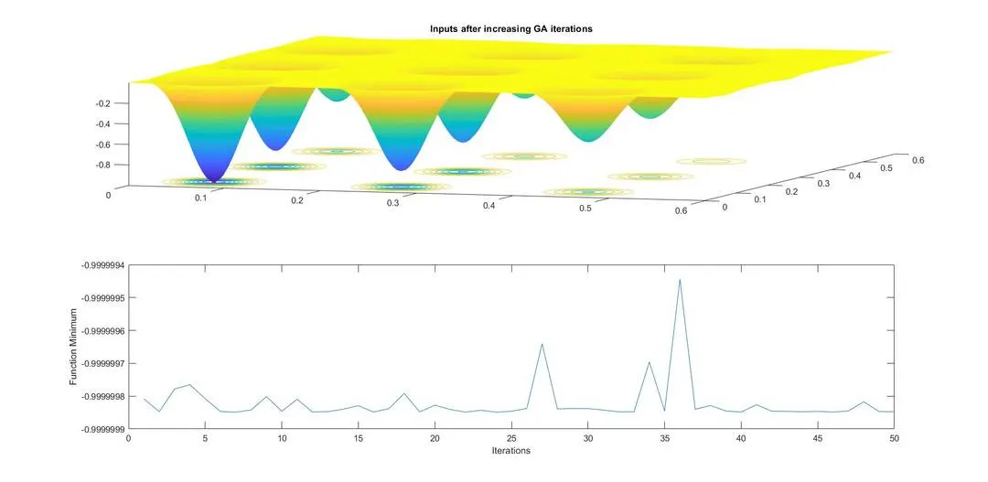
3. Study -3 - Statistical behavior of the function when the inputs are bounded as well as the population size has been specified. The range of the inputs are set to 0-0.2 (as this is where our global maxima are located) and the population size is set to 200. When we run study -3, we observed that we get the same value no matter how many times we run. Hence this result is totally acceptable. The result obtained in study -3 is the global maxima of this function.

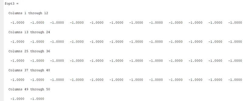
The fopt3 values (the function minimas) for study-3 has been shown below. We can see that the result doesn't vary and we get a constant value no matter how many times we run the program. Hence we can say that the global maxima of our function are 1.