REPRESENTATION OF AN OTTO CYCLE THROUGH P-V DIAGRAM AND TO CALCULATE ITS THERMAL EFFICIENCY IN MATLAB
To write code that can solve an otto cycle and make plots for it
AIM 1 - To write a code to create a PV diagram
AIM 2 - To find the thermal efficiency of the engine.
One very common type of internal combustion engine is the spark-ignition (SI) engine used in automobiles. The Otto cycle is the air standard cycle of such an engine. The sequence of the processes in the elementary operation of the SI engine is given below.
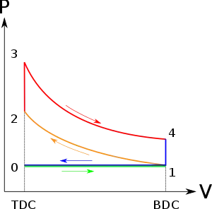
Process 0-1 - The inlet valve is open, admitting the fuel-air mixture into the cylinder at constant pressure.
Process 1-2 - Both the valves are closed, the piston compresses the combustible mixture to the minimum volume. The mixture is compressed isentropically.
Process 2-3 - The mixture is then ignited by means of a spark, combustion takes place and there's an increase in temperature and pressure. Heat is added reversibly at constant volume in this process.
Process 3-4 - The products of combustion do work on the piston and the pressure and temperature of the gases decrease. Work is done by air expanding reversibly and adiabatically in process 3-4. The mixture is expanded isentropically.
Process 4-1 - The exhaust valve opens and the pressure drops to the initial pressure, heat is rejected by air reversibly at constant volume in process 4-1.
Now to write a code to solve an otto cycle, we need to assume certain parameters and inputs. We will be using the below notations for the parameters -
V1 - Volume at state point 1; P1 - Pressure at state point 1; T1 - Temperature at state point 1.
V2 - Volume at state point 2; P2 - Pressure at state point 2; T2 - Temperature at state point 2.
V3 - Volume at state point 3; P3 - Pressure at state point 3; T3 - Temperature at state point 3.
V4 - Volume at state point 4; P4 - Pressure at state point 4; T4 - Temperature at state point 4.
We have been given the following values for calculation -
gamma - the ratio of specific heats = 1.4;
T3 = 1373 K; P1 = 102325 Pa; T1 = 308K;
We also have been given the following engine geometric parameters -
Bore diameter (bore) = 2; Stroke length (stroke) = 4; Connecting rod length(con_rod)= 8; Compression ratio (cr)= 7; Crankpin radius (a) = Stroke length/2; R = ratio of length of connecting rod/crankpin radius(con_rod/a)
Using the above engine geometric parameters, we will be calculating the Volume, V1 at state point 1 and Volume, V2 at state point 2. Then using the ideal gas equations and isentropic relations of pressure, volume, and temperature, we find all the state variables in each state point and plot the PV diagram, and then use those parameters to find the thermal efficiency of the Otto cycle.
Also, as we need to calculate the thermal efficiency of the Otto cycle. The formula for the same is provided below -
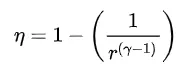
This can be formulated in MATLAB as follows, N being the efficiency of otto cycle -
N = 1 - (1/(cr^(gamma-1)))
% To write a code to solve an otto cycle and make the plots for it
% AIM 1 - To plot a PV diagram

close all
clear all
clc

%INPUTS

gamma = 1.4;
T3 = 1373;

%ENGINE GEOMETRIC PARAMETERS
bore = 2;
stroke = 4;
con_rod = 8;
cr = 7;

%State Variables at state point 1
P1=101325;
T1=308;

% To calculate swept volume and clearance volume
V_swept = pi/4*bore^2*stroke;
V_clearance = V_swept/(cr-1);

V1 = V_swept+V_clearance;
V2 = V_clearance;

%State Variables at state point 2
%We use the isentropic relation between pressure and volume to solve
%P2*V2^gamma = P1*V1^gamma
%P2=P1*(V1/V2)^gamma; As we know cr = V1/V2, we get P2=P1*cr^gamma;
P2=P1*cr^gamma;

%Using ideal gas equation, we can find T2
%P1*V1/T1=P2*V2/T2
T2=(P2*V2*T1)/(P1*V1);

%To calculate Volume and pressure variation during the isentropic
%compression
constant_m = P2*V2^gamma;

%We call a function pistion_kinematics which is shown below
%We calculate the array of volumes during the compression process
V_compression = piston_kinematics(2,4,8,7,180,0);
P_compression = constant_m./(V_compression.^gamma);

%State Variables at state point 3
V3=V2;
%We can use the Pressure-Temperature relationship to solve
%P3/T3=P2/T2;
P3 = (P2*T3)/T2;

%To calculate Volume and pressure variation during the isentropic
%expansion
constant_m = P3*V3^gamma;

%We call a function pistion_kinematics which is shown below
%We calculate the array of volumes during the expansion process
V_expansion = piston_kinematics(2,4,8,7,0,180);
P_expansion = constant_m./(V_expansion.^gamma);

%State Variables at state point 4
V4=V1;
%We use the isentropic relation between pressure and volume to solve
%P4*V4^gamma = P3*V3^gamma
P4 = P3*((V3/V4)^gamma);

%To calculate T4 using ideal gas equation
%P3*V3/T3=P4*V4/T4
T4 = (P4*V4*T3)/P3*V3;

figure(1)
hold on
plot(V1,P1,'*','color','r')
plot(V_compression,P_compression,'color','b')
plot(V2,P2,'*','color','r')
plot([V2,V3],[P2,P3],'color','g')
plot(V3,P3,'*','color','r')
plot(V_expansion,P_expansion,'color','b')
plot([V4,V1],[P4,P1],'color','g')
plot(V4,P4,'*','color','r')

%AIM 2 - To calculate thermal efficiency of the otto cycle
%Consider N to be thermal efficiency

N = 1-(1/(cr^(gamma-1)));

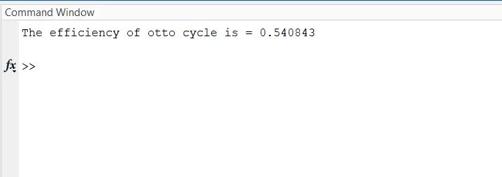
fprintf('The efficiency of otto cycle is = %fnn',N)
So when we execute the code, we will be getting the required outputs as well as a PV plot which is attached below. In the program, we have called a function to calculate the volume and pressure during the isentropic expansion and compression process. Using this we will be tracing the piston volume in the PV diagram.
Before writing the code, we will see the concept which is being used.
We will be using the below-mentioned formula for writing the function -

This is a geometric relationship between the swept volume and clearance volume. θ being the angle made by crankpin radius and R being the ratio of the length of connecting rod and crankpin radius.
Using this we will be able to trace the volume during the isentropic compression and expansion process, where we can see how the volume is changing with respect to the angle made by crank pin radius.
We then calculate the pressure values using the volume trace using the P*V^gamma = Constant relationship. Hence we will be having the values enough to trace the volume and pressure during the isentropic compression and expansion process with which we can connect the state variable coordinates in the PV diagram plotted in the program.
To simplify the above formula while writing the code, we will split it into term1, term2, and term3. θ - theta (for simplicity in the program)
term1 = 0.5(cr-1); term2 = R+1-cosd(theta); term3 = (R^2-sind(theta)^2)^0.5. Hence the equation becomes - v/v_c=1+term1*(term2-term3)
The function is written as shown below -
cr - compression ratio; gamma - the ratio of specific heats;
Below is the code written to find the state variables and to plot the PV diagram, and to find the thermal efficiency of the Otto cycle.
%Function to be called to find the volume change during the compression and
%expansion as mentioned in the above program

function [V]=piston_kinematics(bore,stroke,con_rod,cr,start_crank,end_crank)

a=stroke/2;
R=con_rod/a;

v_s = pi/4*bore^2*stroke;
v_c = v_s/(cr-1);

theta = linspace(start_crank,end_crank,180);

term1 = 0.5*(cr-1);
term2 = R+1-cosd(theta);
term3 = (R^2-sind(theta).^2).^0.5;

[V]=(1+term1.*(term2-term3)).*v_c;

end
Errors found when the program was executed -
1. As shown below, there was an error in line 18 of my function code. The symbol * was missing from the equation. ([V]=1+term1(term2-term3).*v_c ---> [V]=1+term1*(term2-term3).*v_c)
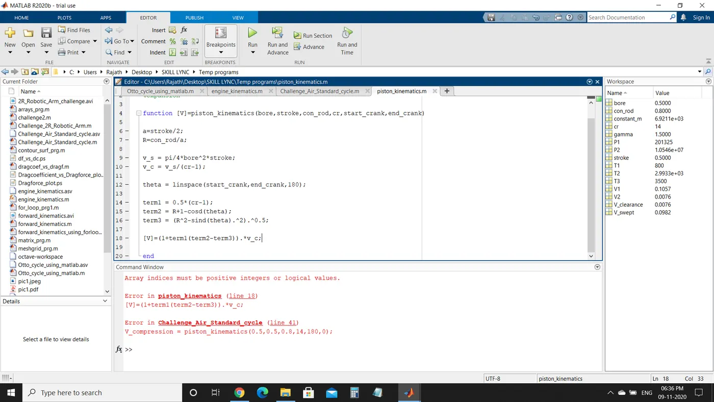
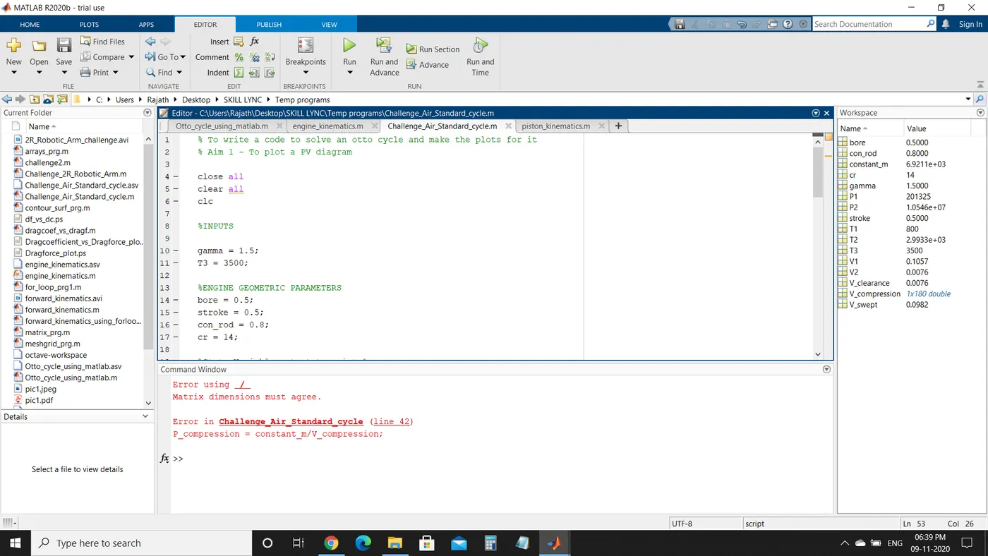
2. As shown below there was an error in line 42. The V_compression is an array and I had missed the '.' before the '/' symbol in the equation ( P_compression = constant_m/V_compression ---> P_compression = constant_m./V_compression)
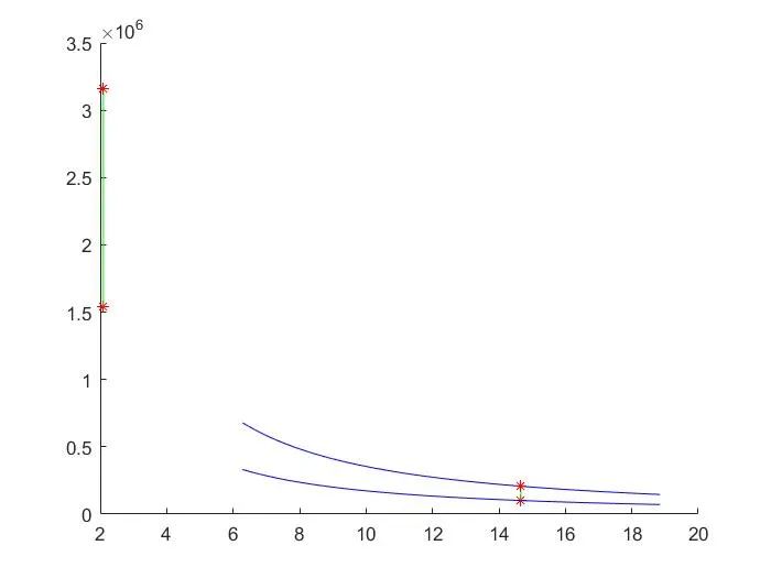
3. As shown below there was an error in the PV diagram.
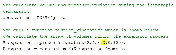
An error was made in the program and is shown below. As I had substituted the wrong value of the Compression ratio both times while calculating the volume trace of isentropic compression and expansion, the graph was plotted incorrectly.
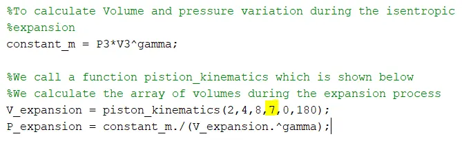
The corrected program with the right value is shown below -
RESULTS -
1. The PV diagram has been plotted and has been attached below as Air_Standard_cycle_RESULT
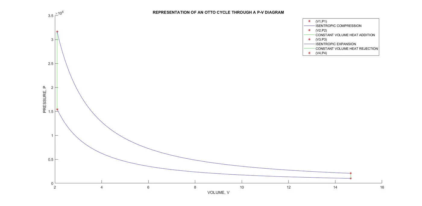
2. The thermal efficiency of the above otto cycle is calculated and is found to be 54.08% which is obtained as an output through the code.