Week 6: Conjugate Heat Transfer Simulation
CONJUGATE HEAT TRANSFER SIMULATION THROUGH A PIPE
Aim:-
To simulate the CHT (Conjugate Heat Transfer) analysis through the pipe with inlet Reynolds number of 7000. And run 3 grid dependence tests to measure the outlet temperature and set the supercycle stage to compare the simulation time.
Theory:-
Conjugate Heat Transfer Analysis:-
The conjugate Heat Transfer (CHT) analysis type allows for the simulation of heat transfer between solid and fluid domains by exchanging thermal energy at the interfaces between them. Typical applications of this analysis type exist as, but are not limited to, the simulation of heat exchangers, cooling of electronic equipment, and general-purpose cooling and heating systems.
Supercycle Stage Interval:-
Super-cycling is the process that the solver of the fluid region is paused until the solver for the solid region converges.
Y+ Wall function:-
The Y+ value is a non-dimensional distance. It is often used to describe how coarse or fine a mesh is for a particular flow pattern. It is important in turbulence modelling to determine the proper size of the cells near domain walls. The turbulence model wall has a restriction on the y+ value at the wall. A faster flow near the wall will produce higher values of y+, so the grid size near the wall must be reduced.
Velocity Calculation:-
Reynolds number (Re) = 7000
Diameter of the Pipe (Fluid region) = 0.03m.
Density of air at 300K = 1.1761 `Kg//m^3`
Dynamic viscosity of air at 300K = 0.00001846 kg/m.s
| `"Re" = (rho*V*D)/("Dynamic viscosity" (mu))` |
`V = (Rexx mu)/(rhoxxD)`
`V = (7000 xx0.00001846) / (1.1761 xx 0.03)`
`"V = 3.66 m/s"`
SIMULATION PROCESS
Part 1 - Grid Dependence test
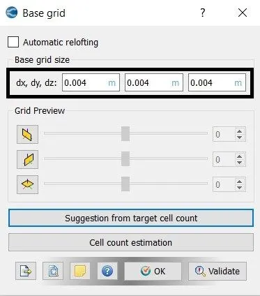
- Mesh Size of 0.004m
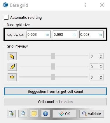
- Mesh Size of 0.003m
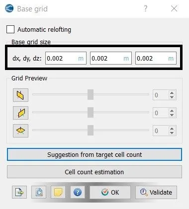
- Mesh Size of 0.002m
Part 2 - Supercycle Stage Time Interval with Base Mesh of 0.004m.
- Supercycle stage interval of 0.01 sec
- Supercycle stage interval of 0.02 sec
- Supercycle stage interval of 0.03 sec
A. Geometry Setup:-
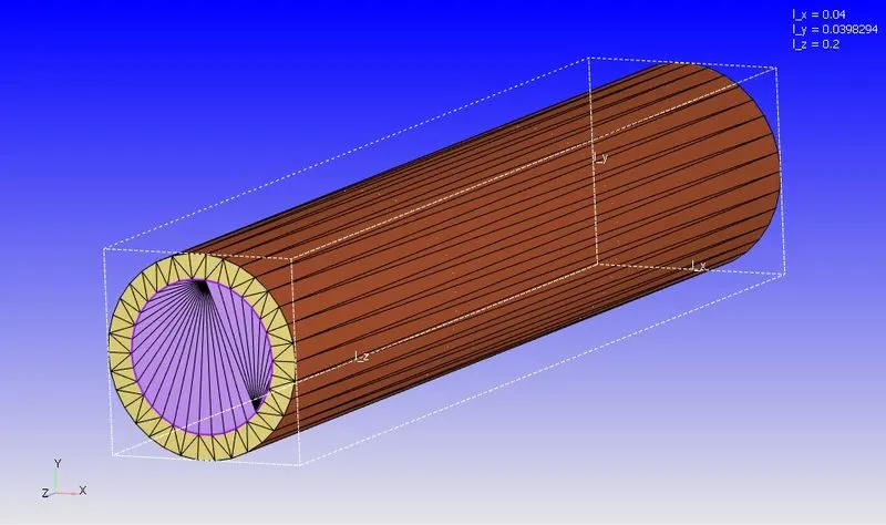
- Create a cylinder with an outer diameter of 0.04m and an Inner diameter of 0.03m.
- Delete the two intersections of the cylinder.
- Close the cylinder thickness by lofted edges.
- Patch the Inlet and Outlet by List of edges.
Geometry:-
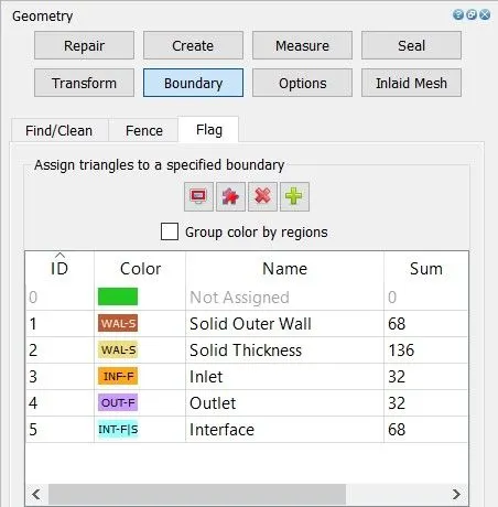
Boundary Flagging:-
B. Case Setup:-
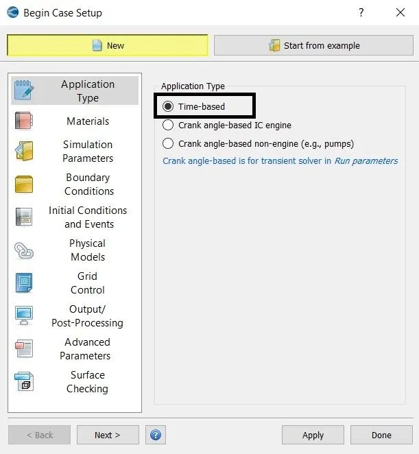
1. Application Type:-
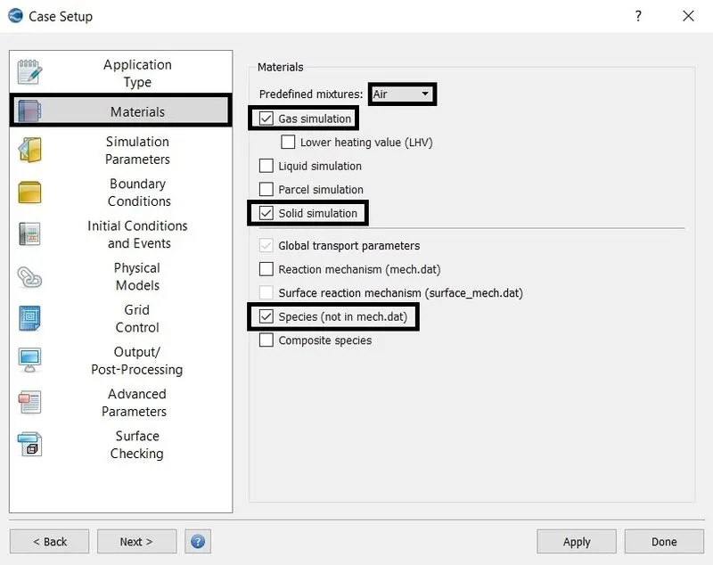
2. Material:-
- Gas simulation
- Solid simulation
- Species - Gas, Solid.
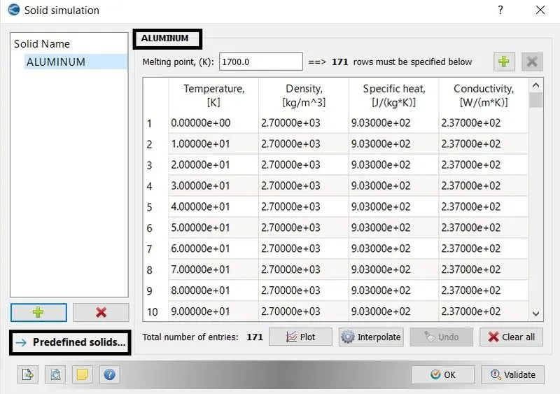
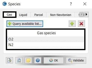
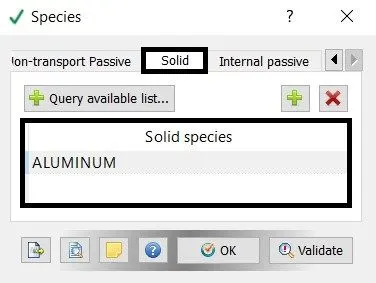
3. Simulation Parameters:-
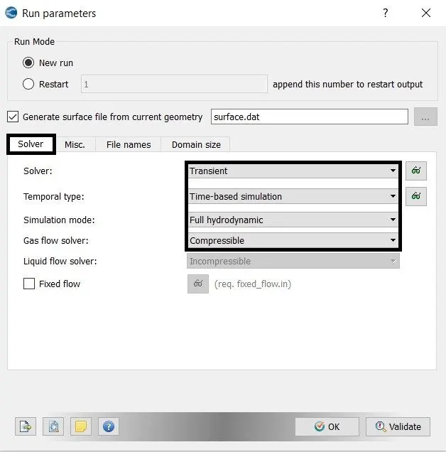
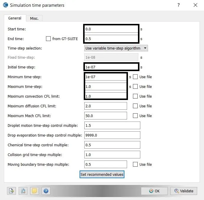
4. Simulation Time Parameters:-
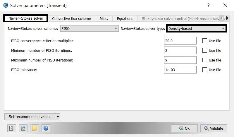
5. Solver Parameters:-
6. Region and Initialization:-
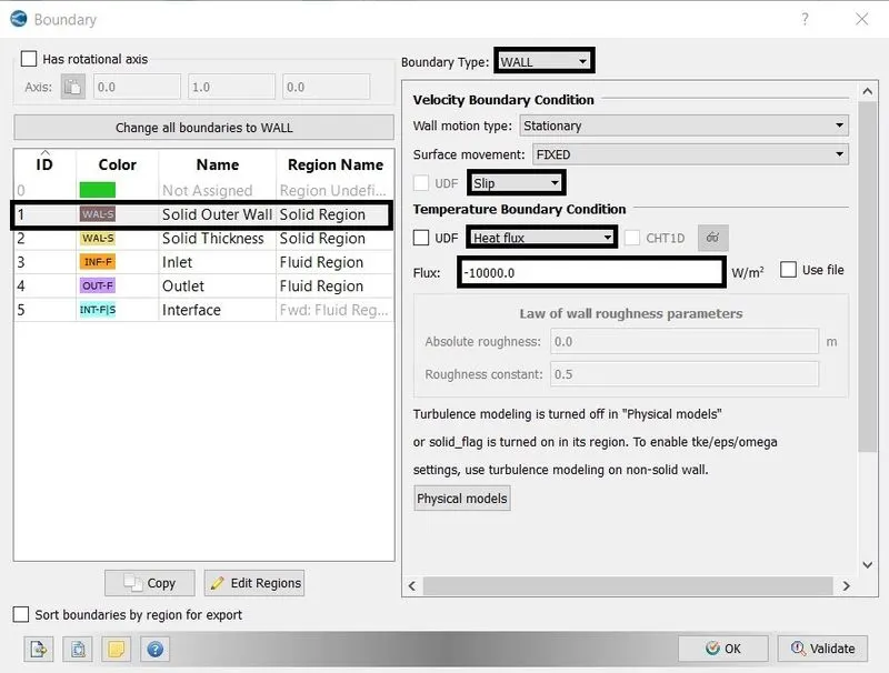
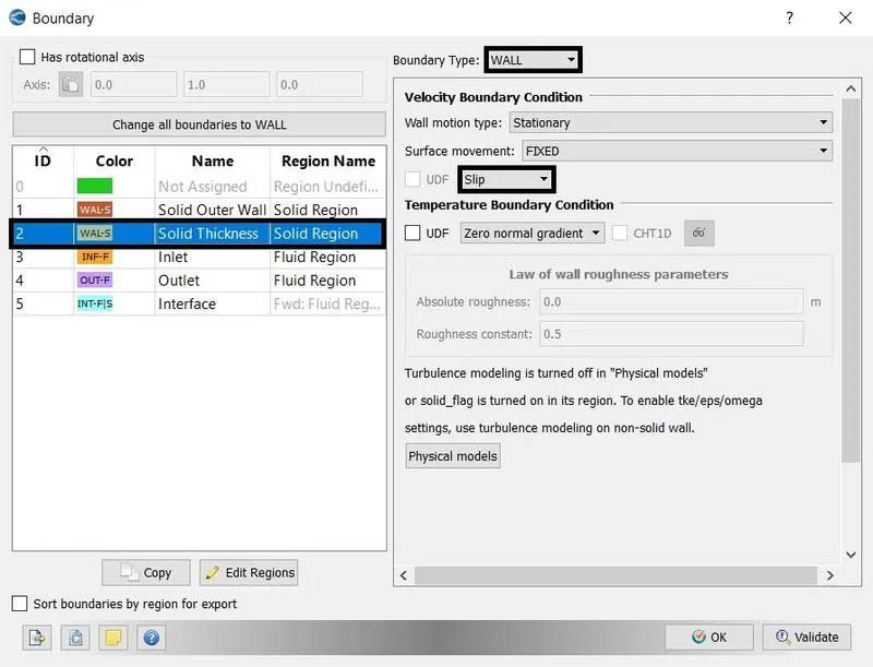
7. Boundary Condition:-
- Solid Outer wall
- Solid Thickness
- Inlet
- Outlet
- Interface
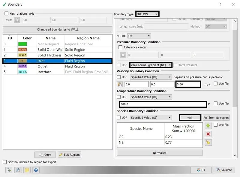
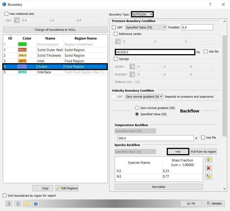
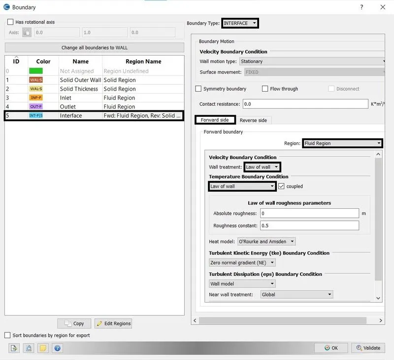
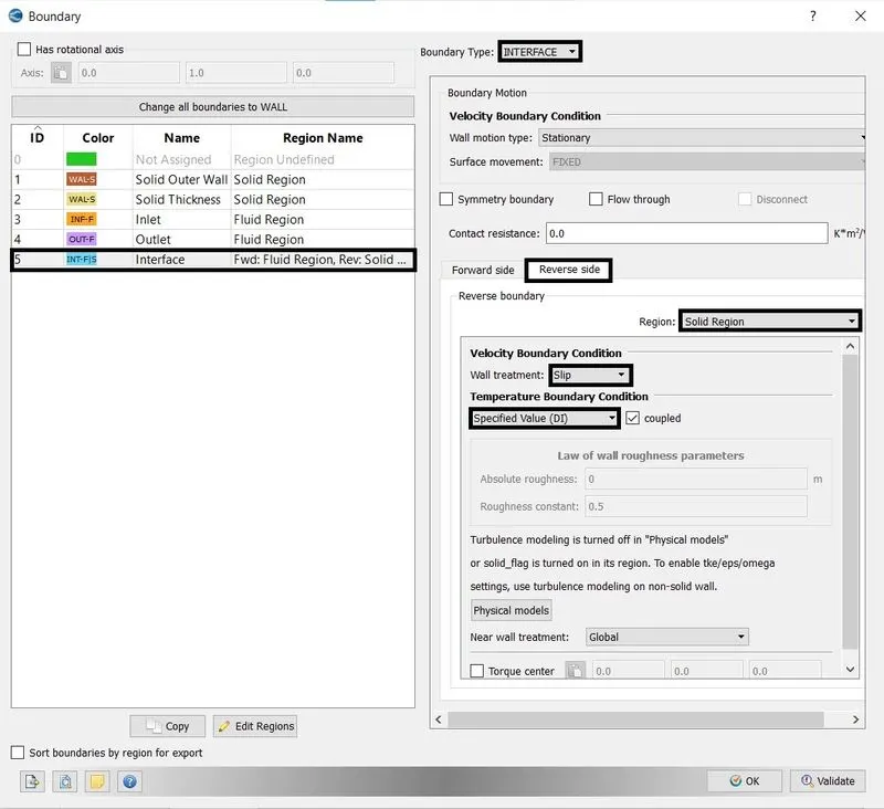
8. Physical Models:-
- Turbulence Model = Reynolds-Averaged Navier-Stroke (RANS), RNG K-epsilon.
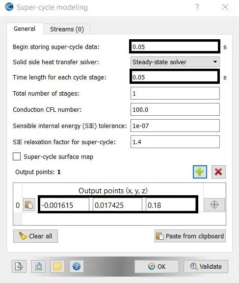
- Supercycle Model
9. Grid Control:-
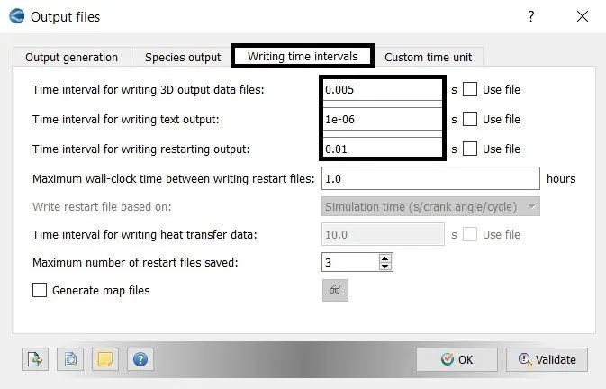
10. Output/Post-Processing:-
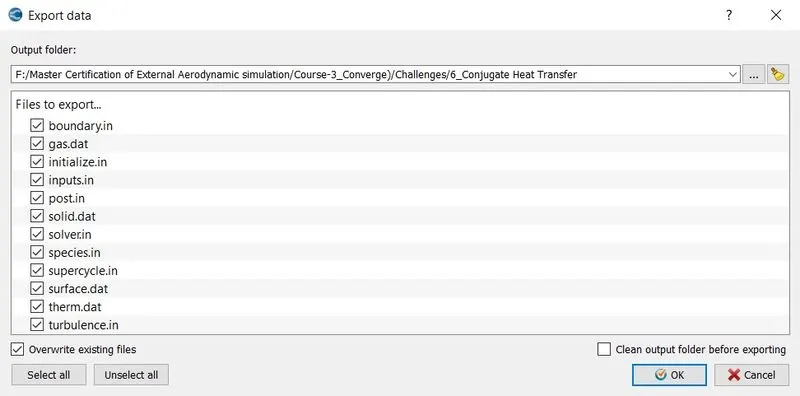
11. Export Data:-
C. Executing the Simulation:-
- The Executable file "mpiexec.exe" and "converge.exe" is pasted in the input files.
- To run the simulation in Cygwin by using the command
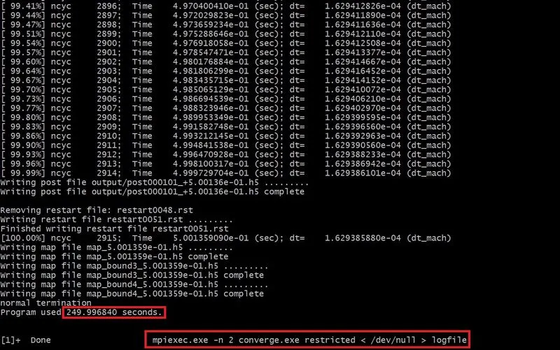
mpiexec.exe -n 2 converge.exe restricted </dev/null> logfile &
- After the simulation is complete, the output files can be converted into paraview VTK in-line binary format to Post-process the result in ParaView.
mpiexec.exe -n 2 post_convert_30_msmpi.exe
*****************************************************************************************
D. Post-Processing:-
Case - 1 (Base Mesh Size of 0.004 m)
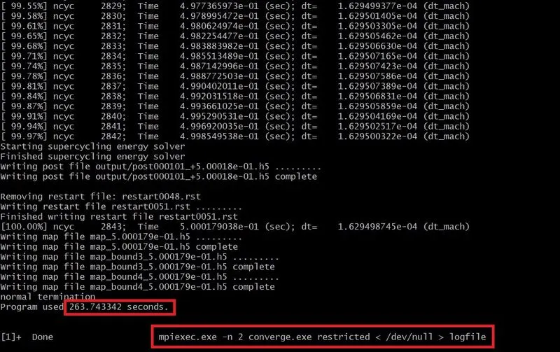
1. Simulation Time:-
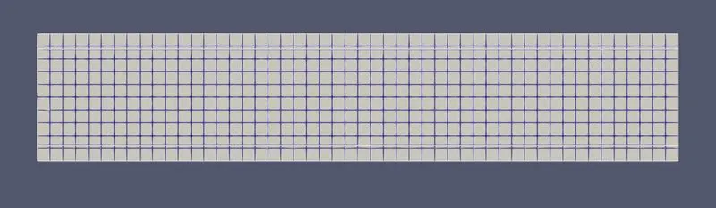
2. Meshing (Surface with edges):-
3. Contours:-
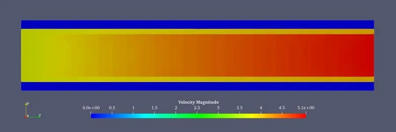
Fig(a). Velocity Contour.
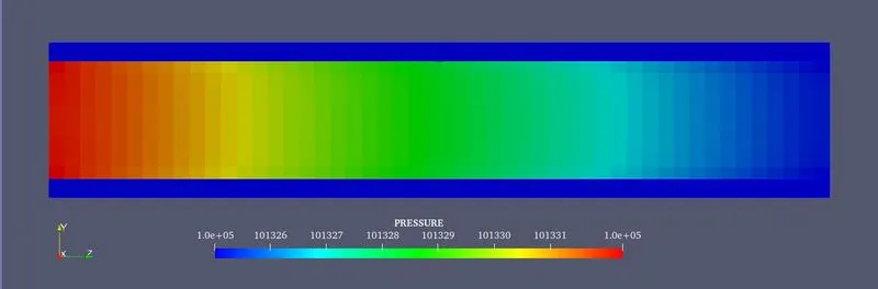
Fig(b). Pressure Contour.
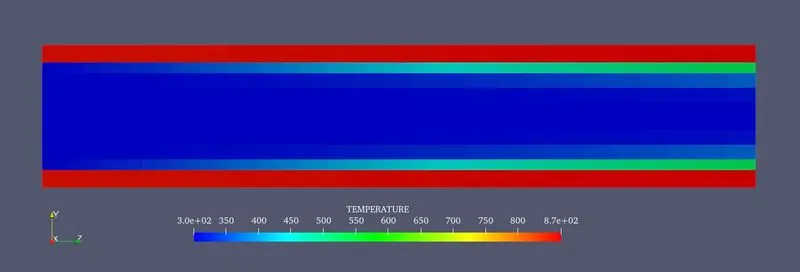
Fig(c). Temperature Contour.
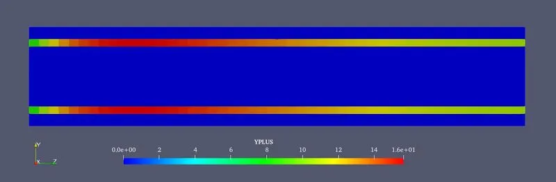
Fig(d). Y+ contours.
4. Line Plots:-
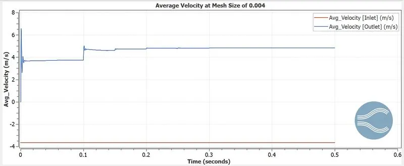
Fig(a). Line Plot of Average Velocity.
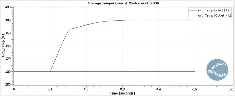
Fig(b). Line plot of Average Temperature.
5. Animation:-
*****************************************************************************************
Case - 2 (Refine Mesh Size of 0.003 m)
1. Simulation Time:-
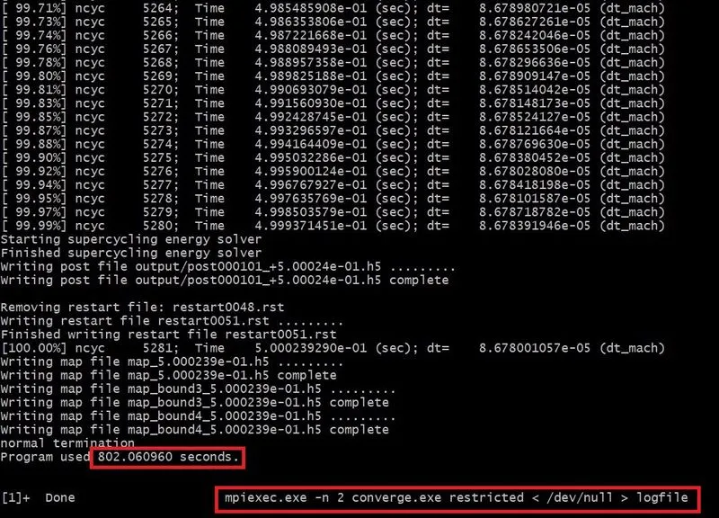
2. Meshing (Surface with edges):-
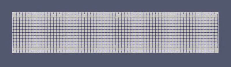
3. Contours:-
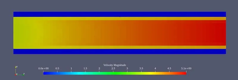
Fig(a). Velocity Contour.
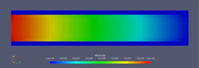
Fig(b). Pressure Contour.
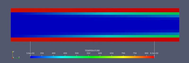
Fig(c). Temperature Contour.
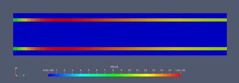
Fig(d). Y+ contours.
4. Line Plots:-
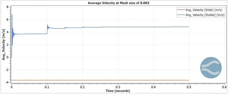
Fig(a). Line Plot of Average Velocity.
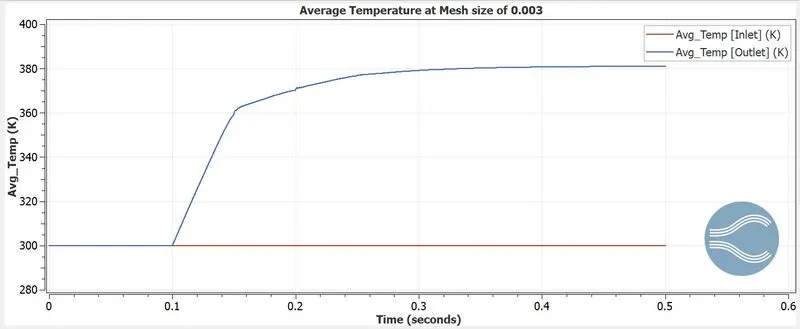
Fig(b). Line plot of Average Temperature.
5. Animation:-
*****************************************************************************************
Case - 3 (Refine Mesh Size of 0.002 m)
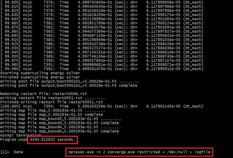
1. Simulation Time:-
2. Meshing (Surface with edges):-
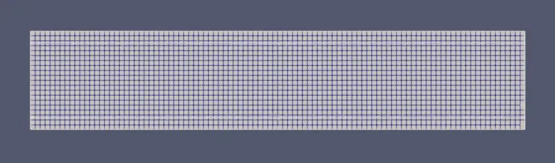
3. Contours:-
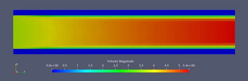
Fig(a). Velocity Contour.
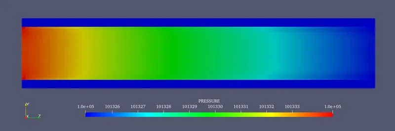
Fig(b). Pressure Contour.
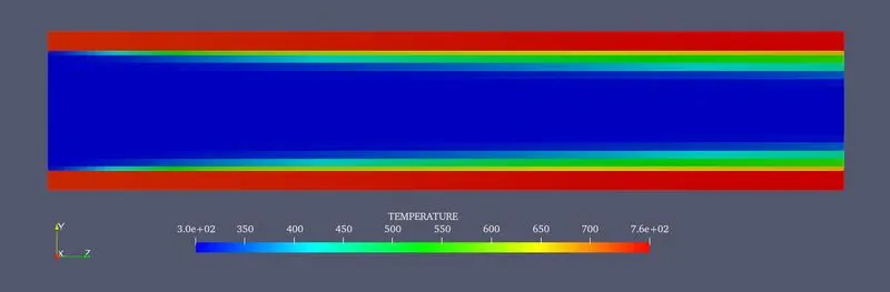
Fig(c). Temperature Contour.
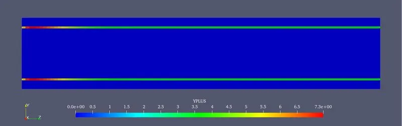
Fig(d). Y+ contours.
4. Line Plots:-
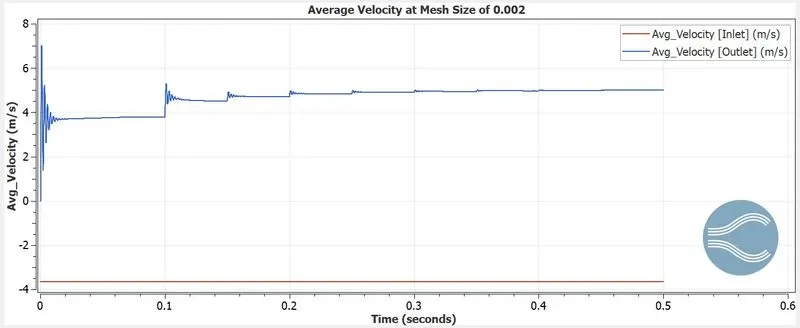
Fig(a). Line Plot of Average Velocity.
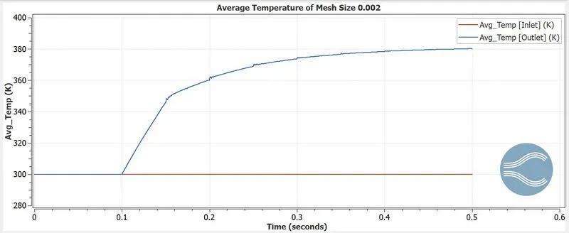
Fig(b). Line plot of Average Temperature.
5. Animation:-
*****************************************************************************************
Case - 4 (Supercycle stage interval of 0.01 sec)
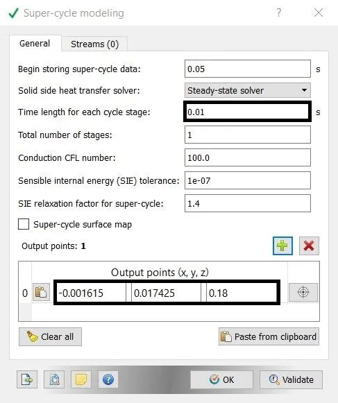
1. Simulation Time:-
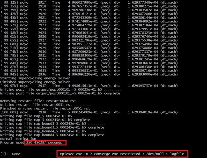
2. Meshing (Surface with edges):-
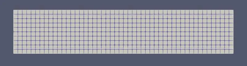
3. Contours:-
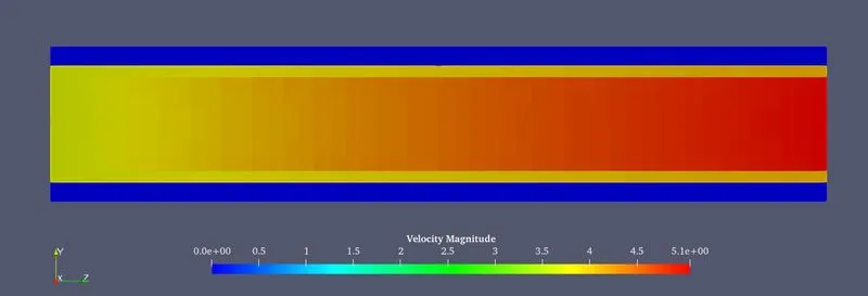
Fig(a). Velocity Contour.
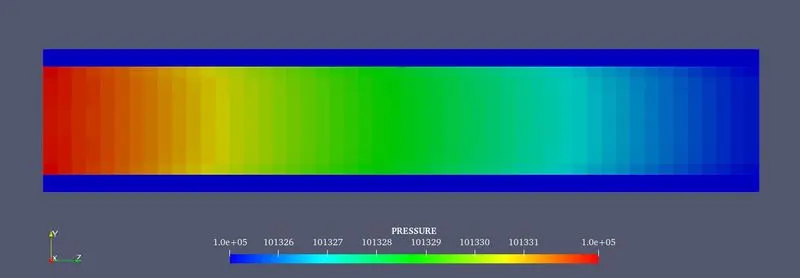
Fig(b). Pressure Contour.
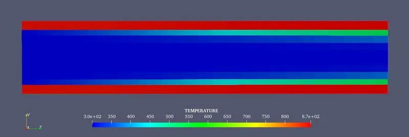
Fig(c). Temperature Contour.
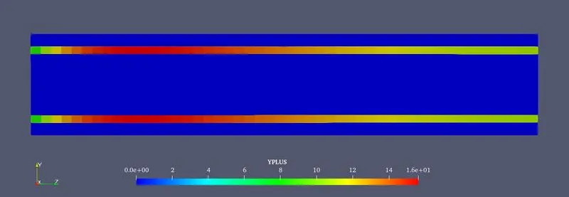
Fig(d). Y+ contours.
4. Animation:-
*****************************************************************************************
Case - 5 (Supercycle stage interval of 0.02 sec)
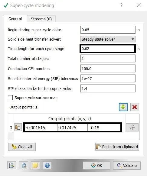
1. Simulation Time:-
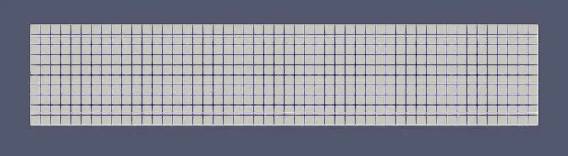
2. Meshing (Surface with edges):-
3. Contours:-
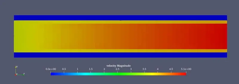
Fig(a). Velocity Contour.
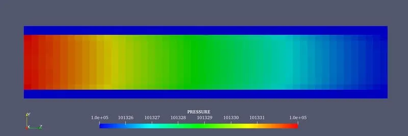
Fig(b). Pressure Contour.
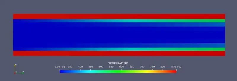
Fig(c). Temperature Contour.
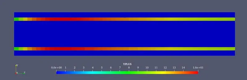
Fig(d). Y+ contours.
4. Animation:-
*****************************************************************************************
Case - 6 (Supercycle stage interval of 0.03 sec)
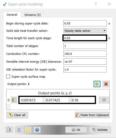
1. Simulation Time:-
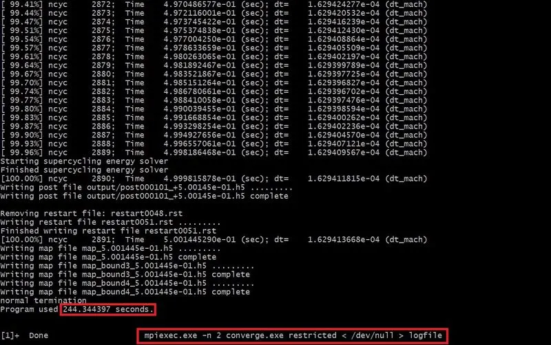
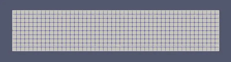
2. Meshing (Surface with edges):-
3. Contours:-
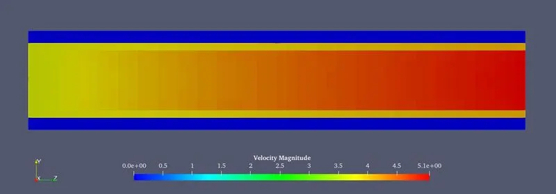
Fig(a). Velocity Contour.
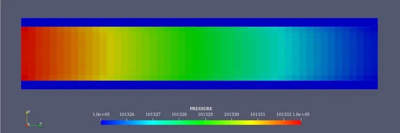
Fig(b). Pressure Contour.
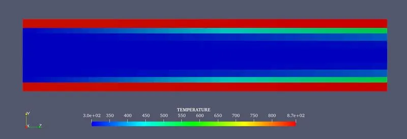
Fig(c). Temperature Contour.
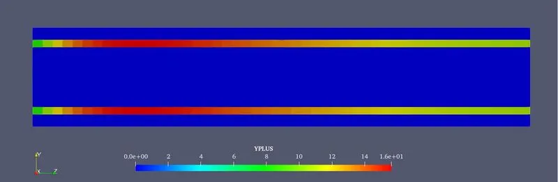
Fig(d). Y+ contours.
.
4. Animation:-
*****************************************************************************************
Comparison of Line Plot:-
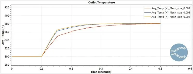
1. Mean Temperature of 3 Mesh Size of 0.004, 0.003, 0.002.
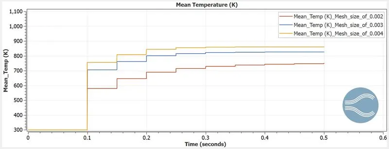
2. The 3 Mesh size 0.004, 0.003, 0.002 of outlet temperature converges to a particular value.
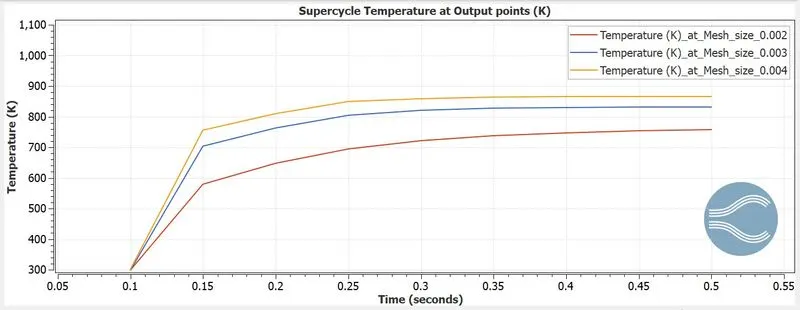
3. Supercycle Temperature at output points of 3 Mesh size.
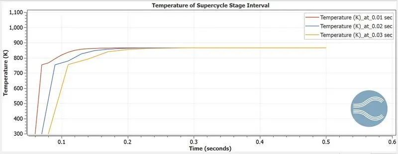
4. Supercycle Temperature at supercycle stage interval of 0.01, 0.02, 0.03 seconds with Baseline mesh.
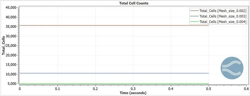
5. Total cell counts:-
Tabulation:-
| Simulation Time (s) | Velocity at outlet (m/s) | Temperature at Outlet (K) | Supercycle Temperature at Outlet (K) | Pressure at Outlet (Pa) | Total Cell Count | ||
| Part - 1 |
Mesh size 0.004 |
263.74 | 4.82 | 380.51 | 865.80 | 101336.67 | 5000 |
|
Mesh size 0.003 |
802.06 | 4.81 | 381.05 | 832.33 | 101336.64 | 10496 | |
|
Mesh size 0.002 |
3430.82 | 4.99 | 380.16 | 757.28 | 101337.92 | 35600 | |
| Part - 2 |
Supercycle stage interval 0.01 sec |
250.45 | 4.82 | 380.52 | 865.94 | 101336.67 | 5000 |
|
Supercycle stage interval 0.02 sec |
249.99 | 4.82 | 380.52 | 865.92 | 101336.67 | 5000 | |
|
Supercycle stage interval 0.03 sec |
244.34 | 4.82 | 380.52 | 865.90 | 101336.67 | 5000 | |
Conclusion:-
- In the CHT simulation, the grid dependence test and super-cycle modelling are used.
- The simulation time and cell count is increased when the grid size is reduced.
- The Outlet temperature is maintained at 380 K.
- Velocity is increased due to reducing of grid size.
- The Pressure outlet maintains nearly to the atmospheric pressure.
- The super-cycle temperature outlet is decreased when the grid size is reduced.
- In the super-cycle stage interval, the simulation time is reduced due to the increase of the super-cycle time interval.
- The velocity, temperature, pressure, supercycle temperature at the outlet doesn't change when the time interval is increased.
- The cell count is also the same in the supercycle stage interval, the simulation time only changed.