Week 6: Conjugate Heat Transfer Simulation

Week 6: Conjugate Heat Transfer Simulation

AIM: -

To set up the conjugate heat transfer through the solid pipe with the specified Reynold number, calculate the velocity and simulation by using Converge 3.0.

INTRODUCTION: -

In the combination of heat transfers in solids and heat transfer in fluids. In solids, conduction often dominates whereas in fluids, convection usually dominates. The term 'conjugate heat transfer' refers to a heat transfer process involving the interaction of conduction within a solid body and the convection from the solid surface to fluid moving over the solid surface. In this heat transfer method, the specified Reynolds number is 7000 with the use of this calculate the velocity of the solid pipe.

PROCEDURE: -

Step 1: Using the software Converge 3.0 select the new project and for creating the geometry select the create option and click the shape, click the cylinder for the inlet circle set as the origin (0,0,0) and set the center point as (0,0,0.015).

Step 2: For the outlet circle set as an origin (0,0,0.2) and the same center point. For the outer circle, inlet is set as (0,0,0) and set the center point as (0,0,0.2) and the outlet circle is set as (0,0,0.2) and set the same center point as (0,0,0.2).

Step 3: Using the repair option-click the delete option and select triangle delete the intersecting triangles from the inlet and outlet on both sides.

Step 4: Now it creates the number of open edges in the diagram, these open edges are easy to find using the diagnosis option.

Step 5: To optimize the open edges select create option and click the triangle and loft edges, set the selection point as by open edges select inlet outer circle for the selection of the first set of edges and inner circle for the select second set of edges and click apply

Step 6: Do the same for the outer side of the cylinder inner and outer circles.

Step 7: For setting the boundary conditions, select boundary 1 as the outer wall and set the name as the solid outer wall.

Step 8: Select the boundary condition 2 set as the solid thickness of the cylinder wall set as a solid side for both inlet and outlet side.

Step 9: Select the boundary condition 3 sets as in the inlet of the cylinder by using the angle method.

Step 10: Select the boundary condition 4 sets as in the outlet of the cylinder by using the angle method.

Step 11: To select the balance inner area of the cylinder is selected as the boundary condition 5 named as interface.

Step 12: Next to set the case set up for the conjugate heat transfer flow of the cylinder.

Step 13: For case, setup selects the Application type is time-based and click ok and done.

Step 14: For the material selection predefined mixture is air and select gas simulation and also the solid simulation also selects the species for the conjugate flow of the problem.

Step 15: For gas, the simulation adds the species as O₂ and N₂ and for the solid simulation add aluminum as the material. For global transport, parameters select the same values and click ok.

Step 16: For the simulation parameters case as run parameter solver is transient and the simulation type is select as full hydrodynamic for the process.

Step 17: For simulation time parameters start time is 0.0 and the End time is 0.5, the Initial time step is 1e-7 and minimum time step is also 1e-7 sec and the maximum time step is set as 1 sec.

Step18: For the solver parameters case select solver type is a pressure-based solver and for the equation section pressure maximum iteration is set as 5000.

Step 19: For the region and initialization set the two regions, one is a solid region the one is a fluid region. For the fluid region ID is 0, the air is added to the flow and for the solid region set as stream, id is 1 and add the species as aluminum and set as a mass fraction is 1.

Step 20: The boundary condition case step is very important for the whole conjugate heat transfer problem. For boundary 1 solid outer wall type is set as a wall for the temperature boundary condition set as heat flux and the value mentioned for that problem is -10000 W/m².

Step 21: For boundary 2 solid sidewall type is set as wall and surface movement of the wall is set as slip.

Step 22: For the boundary 3 Inlet set as wall type is inflow temperature is set as 300 K and the inlet air is added to the condition.

Step 23: For the boundary 4 outlet, the wall type is fixed outflow and the pressure is fixed as specified value and the value is 101325 Pa.

Step 24: For the boundary 5 interface, it can be divided into two sides one is the forward side and reverses side, for the forward side set as a fluid region wall treatment is Law of wall and tke is zero normal gradients. The reverse side set as a solid region wall treatment is set as slip.

Step 25: For the physical modeling add supercycle modeling for the conjugate heat transfer problem.

Step 26: For the supercycle modeling data of the super cycling is set 0.05 and vary the value for three different cases data can be changed as 0.01, 0.02 and 0.03.

Step 27: Time length for each cycle step is set as 0.05 and conduction CFL number set as 100.

Step 28: Internal energy tolerance is set as 1e-7 and the SIE relaxation factor for the supercycle is set as 1.4 and finally click ok and done. To fix the output select one point in the outlet region.

Step 29: For the grid selection process first set the (0.004,0.004,0.004 m). Next for the output and post-processing, post variable selection set species as air O₂ and N₂

And the solid medium selects as aluminum.

Step 30: For output files time interval for 3D output data is 0.005 and text output is 0.1, restart output set as 0.005.

OUTPUTS FOR THE CONJUGATE TRANSFER PROBLEM

These results are should be taken from the initial base and super cycling setup as from the video.

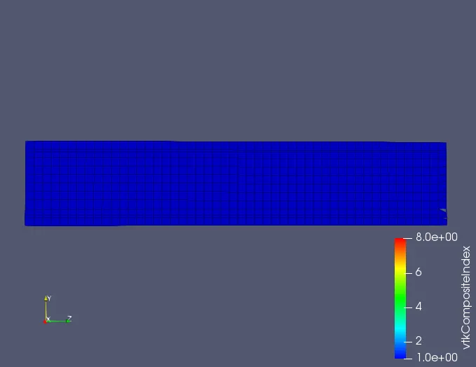
Figure 1. Grid formation of the conjugate heat transfer Cylinder

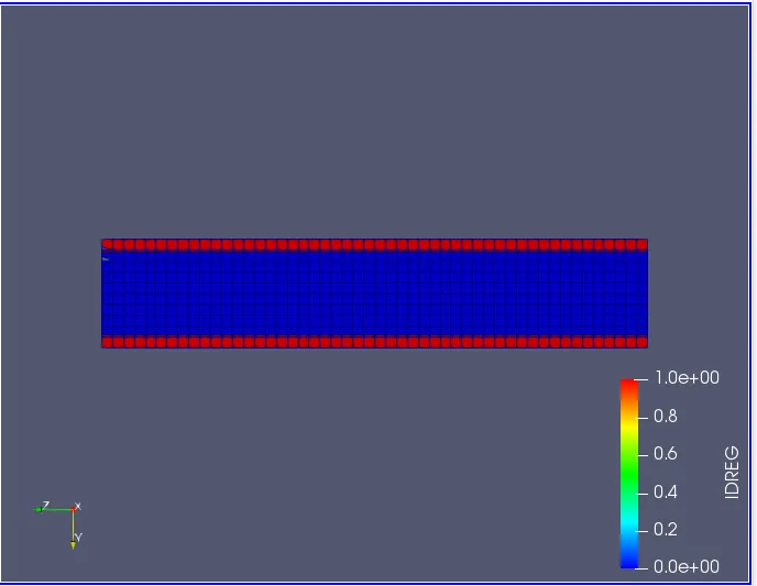
Figure 2. Solid and Fluid region separation of the cylinder

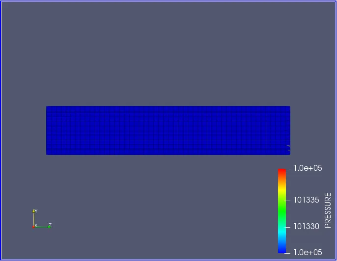
Figure 3. The initial pressure contour of the CHT flow in Cylinder

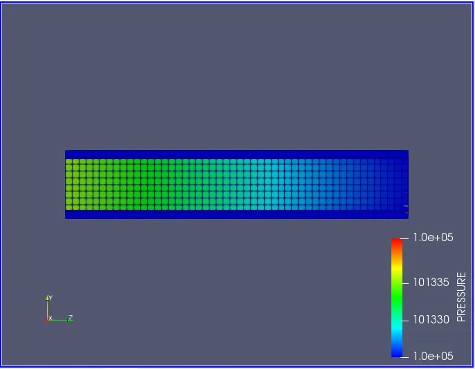
Figure 4. The final pressure of the CHT Flow in Cylinder

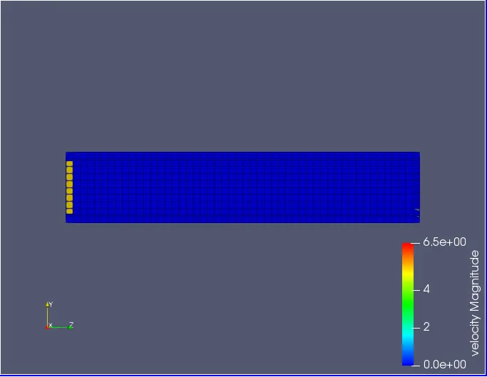
Figure 5. The initial velocity of the CHT flow in Cylinder

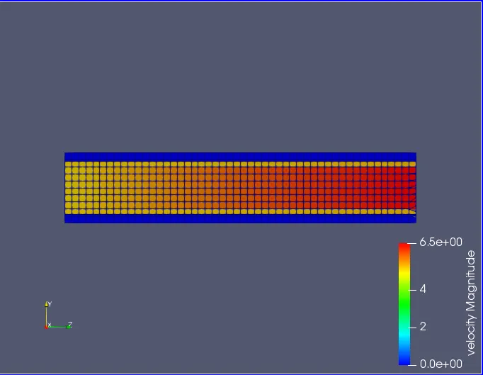
Figure 6. Final velocity contour of the CHT flow in Cylinder

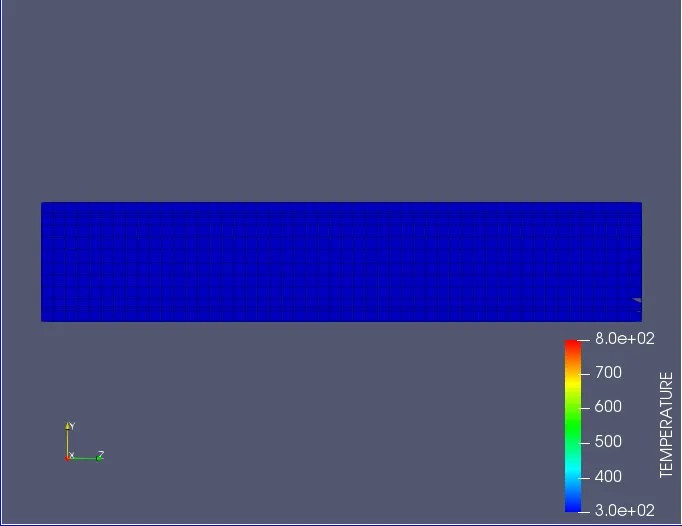
Figure 7. Initial temperature contour of the CHT flow in Cylinder

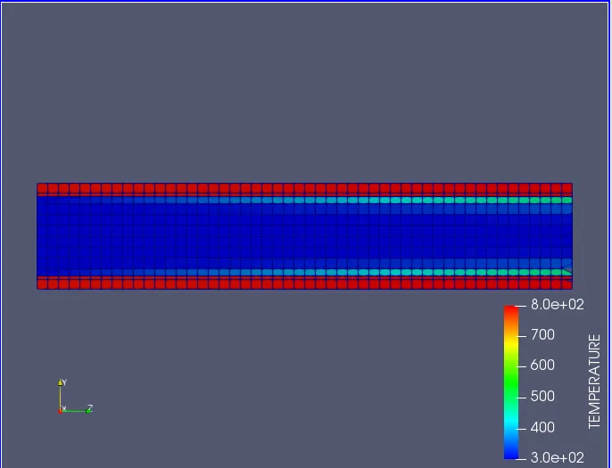
Figure 8. Final temperature contour of the CHT flow in Cylinder

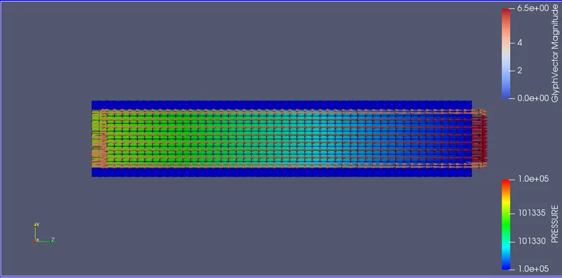
Figure 9. Pressure vector plot of the CHT flow in Cylinder

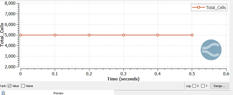
Figure 10. Total cell count for the CHT Flow in the cylinder

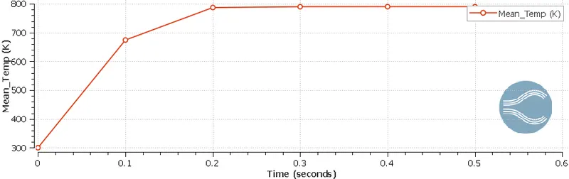
Figure 11. Mean temperature of the 0.05 s super cycle data during the CHT flow

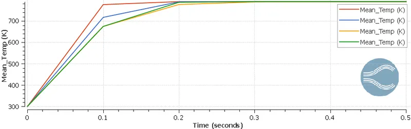
Figure 12. Mean temperature for the various case step of CHT Flow

CALCULATION: -

To find the u_t and v Assume Y+ = 30, Re = 7000, and freestream velocity = 5 m/s

C_f = 0.0576 * Re ^-1/5

= 0.0576 * 7000 ^-1/5

= 0.0576 * 0.1702

C_f = 0.0098039

Ƶ _w = ½ * 0.0098039 * 1.173 * 5²

Ƶ _w = 0.1437 N/m²

u_t = (0.1437/0.12250) ^½

u_t = 0.35 m/s

y = y+ * v / u_t

= 30 * 16e^-6 / 0.35

Y= 0.001371 m or 1.371 mm

Y+ = u/ u_t

u= 10.5 m/s

Result & Discussion: -

1. Run grid dependence test on 3 grids and show that the outlet temperature converges to a particular value.

Outlet temperature selection point :1.7202029244468E-02 3.2156165617900E-03 2.0000000000000E-01

The outlet temperature from the CHT flow is: 800 K

For the super cycling stage interval fix as initial condition 0.05 and given values 0.01, 0.02,0.03 are should be compared the below diagram

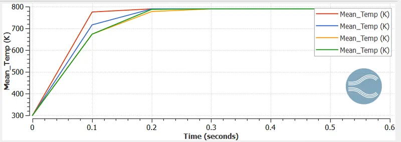
Figure 13: Super cycling stage interval comparing with the other points

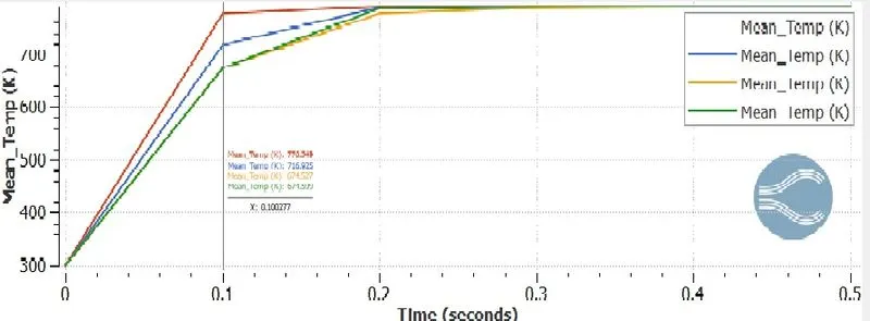
Figure 14: At the time interval of 0.1 sec the mean temperature of the CHT flow

Time interval = 0.1 sec

1. Super cycling Stage Interval is 0.05 = Mean temperature is 776.544 K
2. Super cycling Stage Interval is 0.01 = Mean temperature is 671.599 K
3. Super cycling Stage Interval is 0.02 = Mean temperature is 674.754 K
4. Super cycling Stage Interval is 0.03 = Mean temperature is 716.925 K

CONCLUSION: -

Finally, the Conjugate heat transfer flow problem has been analyzed at various level of the super cycling stage and compared each other for the smooth heat transfer process using Converge 3.0

YouTube Video Link: - https://youtu.be/ObOc7Bscmvs