Week 3: Flow over a backward facing step

WEEK 3: FLOW OVER A BACKWARD STEP

AIM: -

To find the velocity, pressure and mass flow rate distribution of the stepped bar for the various mesh sizes of the element types using converge 3.0.

INTRODUCTION: -

Airflow is the movement of air. The primary cause of airflow is the existence of air. Air particles naturally flow from areas of higher pressure to those where the pressure is lower. Atmospheric air pressure is directly related to altitude, temperature, and composition. If the air passes through the straight pipe it should be a laminar flow, Here the air mixture of oxygen and nitrogen passes through the stepped bar. So that the flow should be varying the velocity, pressure, temperature and mass flow rate in the manner and also here the flow-through in a backward step of the pipe.

EXPERIMENTAL PROCEDURE: -

Step 1: First of all, create import the segmented. stl file or create the stepped pipe as per the requirement of the problem using surface copy comment or repair comment.

Step 2: Check the stepped bar diagram all the triangles are should be closed and all are in the single boundary.

Step 3: Create the various boundary layers for the inlet, outlet, wall and front & back 2-dimensional areas. Select the various type of colors as per boundary and also for each boundary getting the correct layers and number as 1 to 5 and initial-boundary should be zero.

Step 4: Select the normal option and check all the normal directions are should be facing the airflow directions or else choose the transform option to select normal click any one of the triangles and click apply the direction of the normal should be facing the airflow direction.

Step 5: Finally check all are incorrect manner using the diagnosis option and click find all are should be in green color tick mark. All are set to be right.

Step 6: Next case setup, it should be very important for complete the process.

Step 7: Click the case setup and click the Application type, Here the application is not a IC Engine flow it should be a time-based flow, so select the Time-based option and Click ok.

Step 8: Select the materials and select the species option as the nitrogen and oxygen as species.

Step 9: Select the solver run parameters, select the steady-state solver, here the flow passes through the straight pipe only so here mostly the laminar flow occurs. For selecting the solver as Full hydrodynamic it should be used for the real-time process. In that Miscellaneous option select the Steady-state monitor it will be fixing the number of cycles fixed for the flow through the pipe segmentations and un-select the use shared-memory option.

Step 10: In that steady-state solver option have to implement the various dynamic variables as Average temperature, Total pressure and Average density are added. Fix the variables are should be in control of boundary as select the boundary option and finally set as the variables target is output.

Step 11: For the solver parameter option select the Navier stokes solver types as density-based and The equation should be set as pressure, preconditioner option as none. For the steady-state solver controller the CFL limit of the convection is set to be less than 1. It is mandatory for the steady-state control equation flow.

Step 12: Next is defining the boundary condition for the airflow of the stepped bar.

Step 13: Select the inlet boundary and set inflow pressure value for the inlet is 110325 Pa and the outlet boundary set the outlet pressure is 101325 Pa. Here the pressure should be decreased compared the inlet to the outlet. So that the pressure variation created in the stepped bar. Necessary to add the inlet and outlet air for the system as N₂ = 0.77 O₂ = 0.23.

Step 14: The front and back two-dimension walls are selected as 2D constraints, they does not create any impact on the flow of the airflow through the duct.

Step 15: The boundary of Top and Bottom wall select the walls of the flow and here set the option as law of the wall. It should be creating some deviations in the flow and also the wall embedding also enabled for the wall structure.

Step 16: After defining the boundary conditions must select the region of the boundaries. create one region as Volumetric region user-defined and set as all the boundaries are under the selected region.

Step 17: Next as initial conditions and events, the one region is set for all the boundary conditions.

Step 19: The physical modeling set up select without any modification for the current flow.

Step 20: For the grid control option to set a problem as various steps in the grid control plays a major role and also its affect the accuracy of the problem solution. In that base gird option also select the boundary embedding option. This embedding option should be creating the number of elements that should be created the complicated shape into a smooth surface. So that its uses to attain the accuracy result in the flow-through pipe problems.

Step 21: The selection of gird also makes the increment of elements in the given diagram. Select the gird in is for dx = 0.002 dy = 0.002 dz = 0.002 for the first case.

Step 22: Post variable selection, in this option, select the number of variables and set of variables to be displayed in the entire result.

Step 23: Output files, this is the important step for the categories the results, so that post variable selection option is must to be set below 200 to attaining the minimum output files as 15.

Step 24: Time interval for writing 3D output data files: 100 Cycles

The time interval for writing text output: 1.0 Cycles

The time interval for writing restarting output:100 Cycles

This should create an output file maximum of 150 files to get high accuracy.

EXPLANATION FOR THE RESULT: -

For the Flow over the backward step result contours for the velocity, temperature and pressure and pressure vector plot are shown below: -

Pressure Contour Plots: -

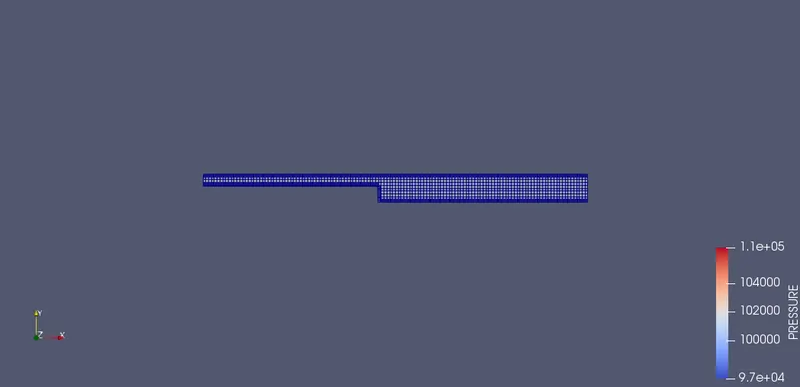
Fig 1. Initial Pressure contour plot for case 1 mesh grid value is 0.002 = 9.7e+4 Pa

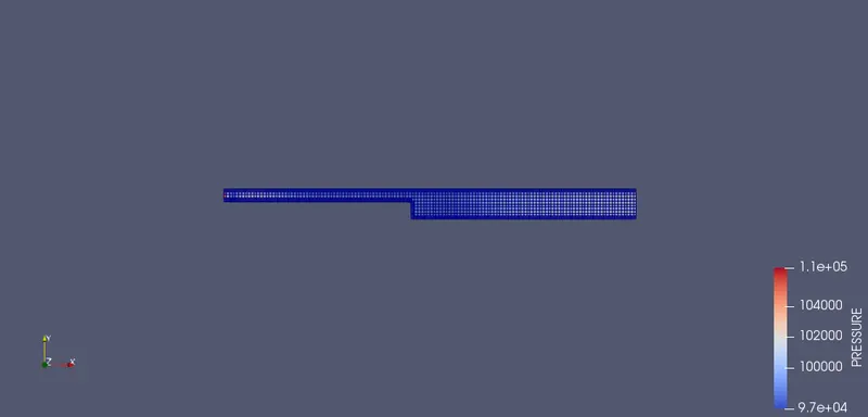
Fig 2. Final Pressure contour plot for case 1 mesh grid value is 0.002 = 1.1e+5 Pa

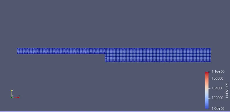
Fig 3. Initial Pressure contour plot for case 2 mesh grid value is 0.0015 = 1e+5 Pa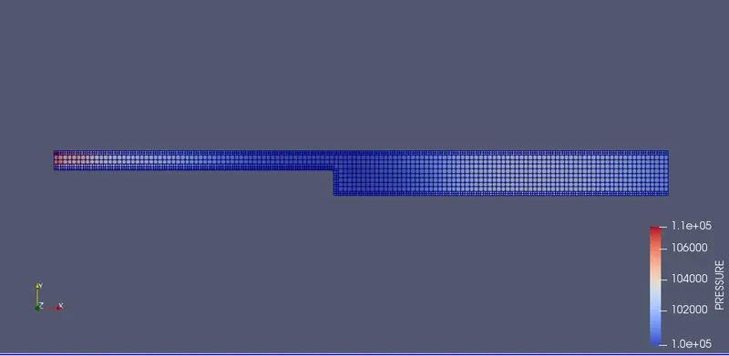

Fig 4. Final Pressure contour plot for case 2 mesh grid value is 0.0015 = 1.1e+5 Pa

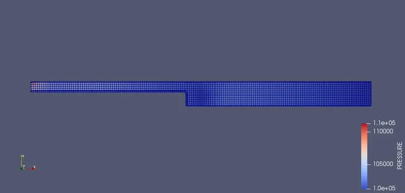
Fig 5. Initial Pressure contour plot for case 3 mesh grid value is 0.0012 = 1e+5 Pa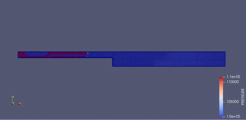

Fig 6. Final Pressure contour plot for case 3 mesh grid value is 0.0012 = 1.1e+5 Pa

Velocity Contour Plots: -

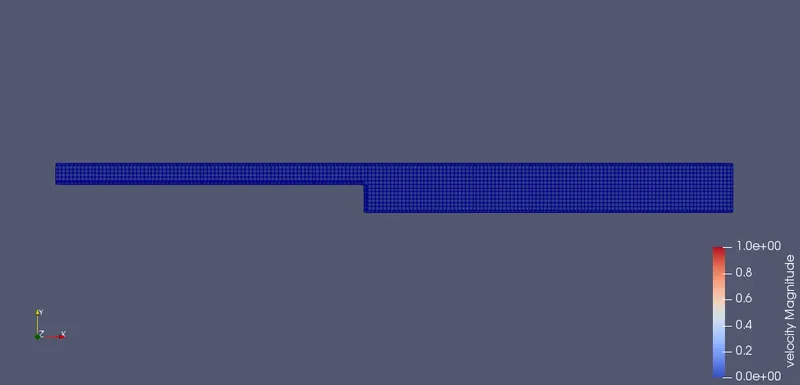
Fig 7. Initial Velocity contour plot for case 1 mesh grid value is 0.002 = 0.0e+0 m/s

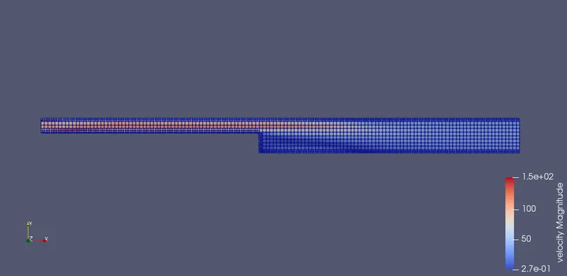
Fig 8. Final Velocity contour plot for case 2 mesh grid value is 0.002 = 1.2e-3.8 m/s

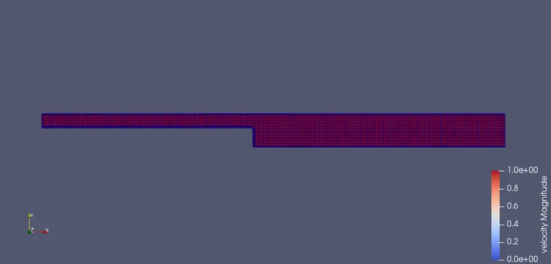
Fig 9. Final Velocity contour plot for case 3 mesh grid value is 0.0015 = 1.5e+2 m/s

Temperature contour Plots: -

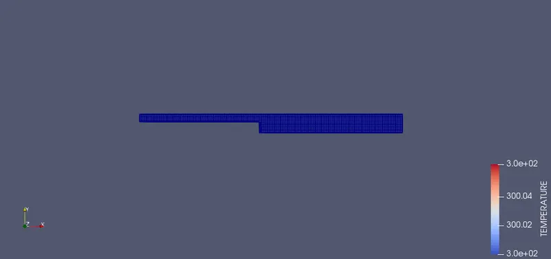
Fig 12. Initial temperature contour plot for case 1 mesh grid value is 0.002 = 300 K

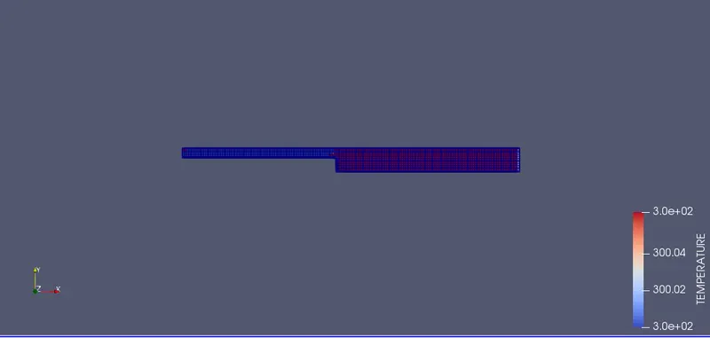
Fig 13. Initial temperature contour plot for case 3 mesh grid value is 0.0012 = 300 K

Pressure Vector Contour Plots: -

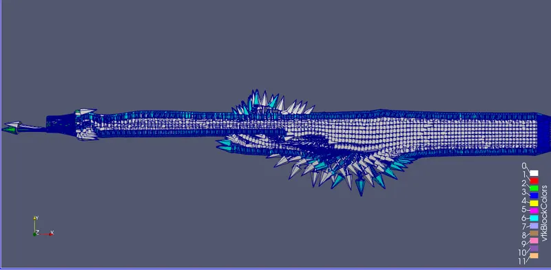
Fig 14. Pressure Vector contour plot for case 1 mesh grid value is 0.002

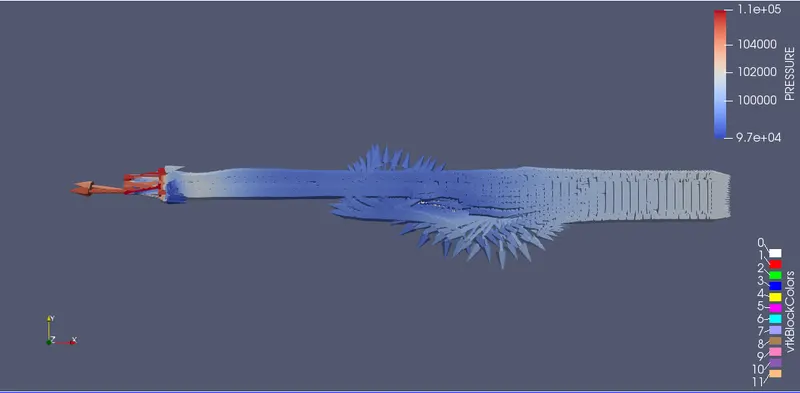
Fig 15. Pressure Vector contour plot for case 2 mesh grid value is 0.0015

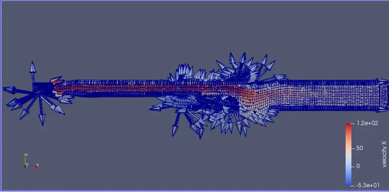
Fig 16. Pressure Vector contour plot for case 3 mesh grid value is 0.0012

From the above results

The below values are to be set and standardize for the all the grid mesh value problems

The inlet Pressure for the inlet flow = 110325 Pa

The outlet pressure for the outlet flow = 101325 Pa

Top and Bottom walls are should be set as Law of wall it should create some impact in the flow.

Simulation time are should be fixed as No of cycles as 15000 Cycles

Minimum initial time of simulation 1e-6 sec

Maximum time of simulation 1 sec

Time interval for writing 3D output data files: 100 cycles

Time interval for writing text output: 1e-9

Maximum number of restart files saved 3

DETAIL OF THE RESULT: -

For the flow through the backward step pipes the temperature contour plot for the initial and final plot is remaining same as 300⁰C.

To fix the various grid base levels as 0.002, 0.0015 and 0.0012

The maximum values of the simulation period steps are should increase as 8, 32 and 150.

It should be increased the number of elements present in the stepped bar and increase the accuracy of the results to reduce the gird values.

For the result initial values are should be present in the problem for the velocity, pressure and mass flow rate is 0.0e+0, 9.7e+4 and 1.1e+3. The final values of the velocity, pressure and mass flow rate is 1.5e+2, 1.1e+5 and 10.1e+3. For the three cases and vector plots are shown that are should be in different directions.

The boundary embedding also used for this problem the embedding creates the complexity shapes as into the form of detail element structure. In this case the bar has been refined 1 times and only 1 cell is at a particular refinement level from the boundary.

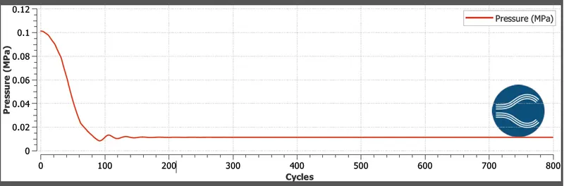
Fig 17. Initial Pressure curve for the lowest gird segmentation problem

YouTube video link: https://youtu.be/SWsUQWgHjp0