Week 5: Prandtl Meyer Shock problem
Week 5: Prandtl Meyer Shock problem
AIM: -
To create the supersonic and subsonic flow through the rectangular object and analyze the shock problem with suitable boundary conditions by using Converge 3.0.
INTRODUCTION: -
In this shock wave problem, there are three different types of boundary conditions are should be used. For the inlet flow Dirichlet boundary condition and the outlet flow Neumann boundary condition are should be used. For the Computational fluid dynamics problems, these two boundary conditions are mostly used. Also, in this problem the two different types of flows are can be used for analyzing the shock problem. The subsonic and supersonic conditions of flows are used in the problem and also two different types of SGS conditions are used. Finally, shock wave areas were analyzed by using the converge 3.0 software.
Subsonic Flow: -
Subsonic if the Mach number is less than 1 at every point. Moreover, since the flow velocity is everywhere less than the speed of sound, disturbances in the flow (say the sudden deflection of the trailing edge of the airfoil.
Supersonic Flow: -
When the Mach number is greater than 1.0 or V is greater than C, then the flow is called Supersonic Flow.
Different types of boundary conditions: -
Boundary conditions are constraints necessary for the solution of a boundary value problem. ... Boundary value problems are extremely important as they model a vast amount of phenomena and applications, from solid mechanics to heat transfer, from fluid mechanics to acoustic diffusion. Boundary conditions are generally three types. They are Dirichlet boundary condition, Neumann boundary condition and mixed boundary condition.
Dirichlet boundary condition: -
In fluid dynamics, for the inlet boundary has the no-slip condition for viscous fluids states that at a solid boundary, the fluid will have zero velocity relative to the boundary. Dirichlet boundary condition may also be referred to as a fixed boundary condition. Here the inlet Mach number is 2. So that for the inlet flow Dirichlet boundary condition is used.
T=1 for y=1, and 0≤x≤1
T=0 for x=1, and 0≤y<1
Neumann boundary condition: -
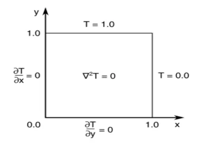
Figure 1: Rectangular domain with homogeneous Neumann boundary conditions
∂T/∂x=0 for x=0, and 0<y<1
∂T/∂y=0 for y=0, and 0<x<1
Where would be the derivative of the unknown is given in the boundary and also the high number of grids used for the simulation, in that area of simulation the Neumann boundary conditions are used. This type of boundary conditions is common and specified mostly where outlet velocity is known. The flow attains a fully developed state where no change occurs in the flow direction when the outlet is selected far away from the geometrical disturbances. In such region, an outlet could be outlined and the gradient of all variables could be equated to zero in the flow direction except pressure.
Shock wave: -
Change of pressure in a narrow region traveling through a medium, especially air, caused by the explosion or by a body moving faster than sound is called a shock wave and the Mach number of the flow is greater than 1.
There are three types of the shock waves
- Electromagnetic shockwave
- Piezoelectric shockwave
- Electrohydraulic shockwave
Temperature flow through the rectangular duct: -
Step 1: Creating the 3D model of the rectangular duct using the modeling software in the format of .stl file.
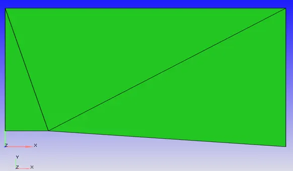
Figure 2: 2D rectangular duct
Step 2: Using the converge studio index open the .stl rectangular duct and add a single boundary.
Step 3: Select the boundary command click add boundary 5 more boundaries are added.
Select the inlet and outlet boundaries are 1 and 2 respectively.
Step 4: Select the total top and bottom surface is boundary 4 named as side walls.
Step 5: Next to select the front and backside wall, select the front side 2-dimension wall is a boundary number is 3 and the front side 2 dimensional wall is set as the boundary number 3.
Step 6: After the separation of all boundaries click the setup option and click the Application type and select the time based option, here the problem was steady state condition, it’s not a IC engine problem its depends on the time only.
Step 7: Next to select the materials, the predefined mixture was air and select the option as gas simulation, add the species option and select ok.
Step 8: Next for the global transportation parameters as default option is selected and the species option click and add the O2 and N2 are the airflow inlet gases.
Step 9: Next for the simulation parameters click the solver as steady state solver, it’s the necessary condition for this case. For the miscellaneous option select the select the steady state monitor option.
Step 10: Next click the steady state monitor option add the various variables as Average temperature, Total pressure, average velocity and select the target type is boundary also select the target is outlet for the condition.
Step 11: Next for the important step, simulation time parameters set the start time is 0.0 Cycle, End time is 15000 cycles, Initial time step is 1e-7, Minimum time step is 1e-7 and the maximum time step is 1 second.
Step 12: Next for the solver parameters Navier – stokes solver type is pressure based and pressure precondition is none and steady- state solver Initial PISO convergence criterion multiplier value is must below 1 set the value is 0.5.
Step 13: Next to select the boundary conditions for the flow as, first for the inlet flow pressure boundary condition is set as zero normal gradient and the velocity boundary gradient is set as specified value (DI) 680 m/s. It’s very high compared to the light velocity. So that the flow Mach number is 2 and the flow is supersonic flow.
Step 14: For the temperature boundary condition the temperature value is set as 286.1 K and the air added to the inlet boundary condition.
Step 15: For the outlet select the pressure set as Neumann boundary condition like the pressure boundary condition is zero normal gradient and the velocity boundary condition also zero normal gradient specified value for the back flow is selected and the temperature boundary condition the temperature value is set as 300 K and air is added to the outlet flow simulation.
Step 15: The side walls like top and bottom are should be simply set as two dimensional walls.
Step 16: The front and back two dimensional walls are selected stationary and slip wall condition.
Step 17: For the regions and initialization add the new region named as region 0. In that region fix the velocity value is 680 m/s and temperature value is 300K. The air is to be added to the region.
Step 18: For the base grid selection the grid value is set to be 0.8 m for all the directions.
Step 19: In this grid selection also added an embedding selection, it’s very useful to separate the elements in the complicated shapes in an ahead manner. The fixed embedding creates the minimum size of the elements creations.
Step 20: Next for the post variable selection select the two species in the field of mass fraction and select ok.
Step 21: Time interval for the 3D output data files is 1000 Cycles and Time interval for writing restarting output is 1000 cycles are should be selected in the field of post processing selection.
Step 22: In the base gird selection added the another one condition is adoptive mesh refinement, in that condition wherever the flow increases that places the grid size is reduced as per the refinement calculation with the requirement of the flow.
Step 23: For the AMR, minimum cell calculation is set as 1, Maximum cells are set as 200000, embedded frequency is 1, releasing frequency is above 25.
Step 24: Place the active region as region 0 and the temperature and velocity are should be selected for the SGS Maximum embedding level is 3 and the sub grid criterion is set as 2.5 for the case 1 and that 0.5 for the case 2.
Step 25: Finally export all the data into the selected folder and also copy the mpiexec and converge-intelmpi files into the folder and run the program.
Step 26: Also post-processing is done using the converge 3.0 simulation process .vtm group file also created.
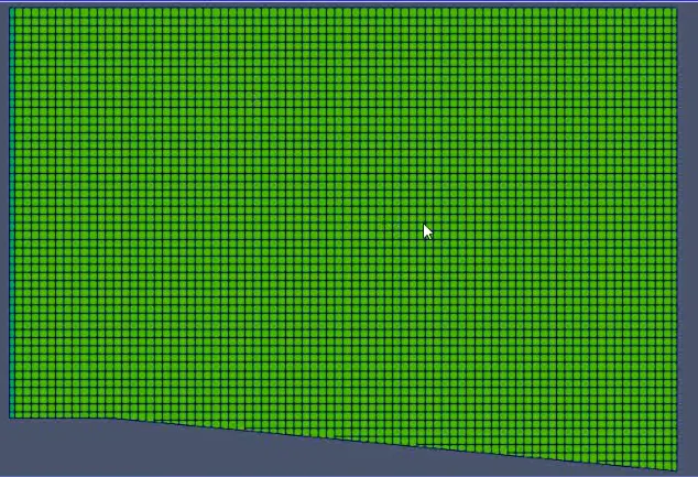
Figure 3: Mesh with edges of the rectangular duct
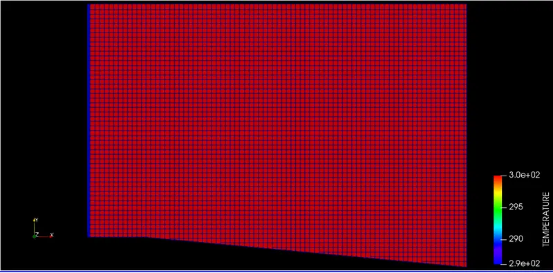
Figure 4: Initial temperature contour for the supersonic flow through the duct
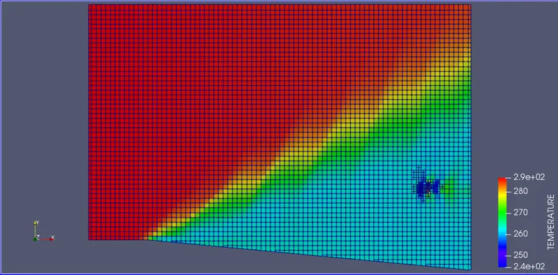
Figure 5: Supersonic flow through the rectangular duct
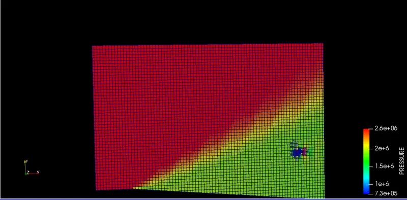
Figure 6: Pressure at the middle range of the supersonic flow
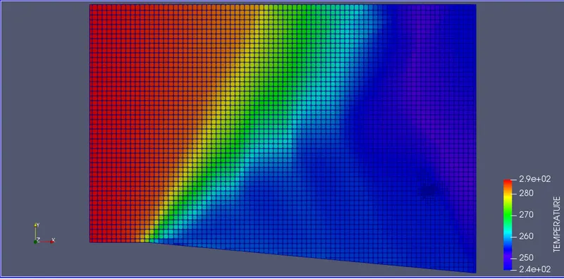
Figure 7: Temperature flow through the final stage of supersonic flow
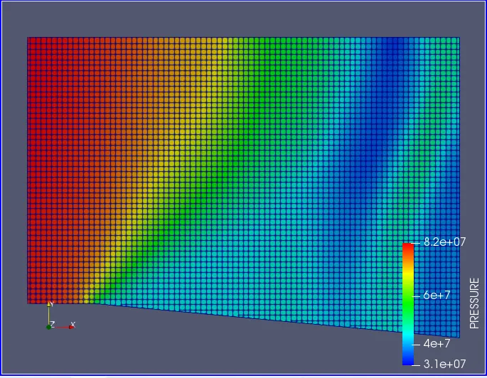
Figure 8: Supersonic flow through the rectangular duct
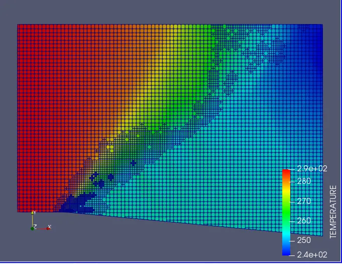
Figure 10: SGS creation during the supersonic flow through the rectangular duct
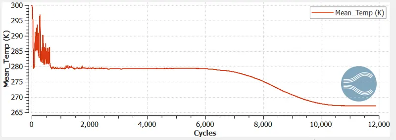
Figure 11: Mean temperature flow through the rectangular duct
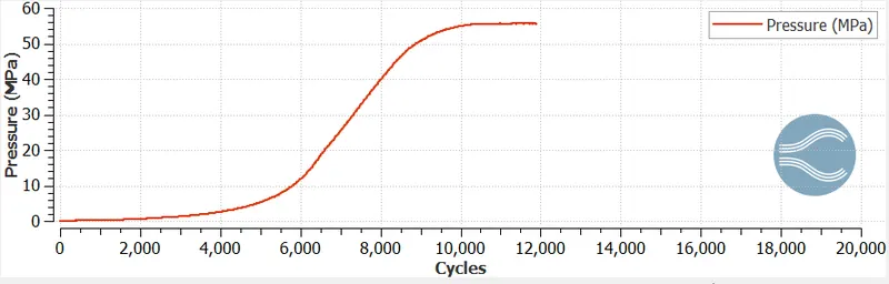
Figure 12: Pressure flow through the rectangular duct during supersonic condition
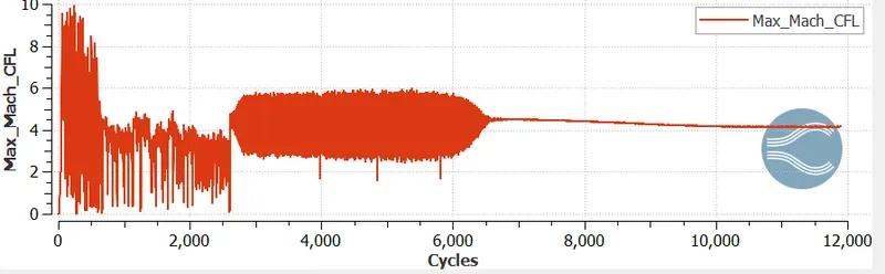
Figure 13: Mach CFL during the supersonic simulation
SUBSONIC FLOW: -
A subsonic wave is a wave that is traveling slower than the speed of sound and a supersonic waves travels faster. By definition, a sound wave travels at the speed of sound which varies depending on the medium through which it's traveling.
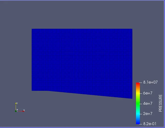
Figure 14: Initial pressure during the subsonic flow simulation
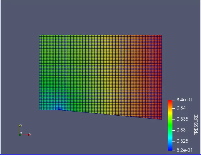
Figure 15: Final pressure contour during the subsonic flow simulation
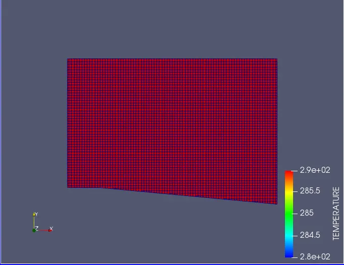
Figure 16: Initial temperature contour during the subsonic flow simulation
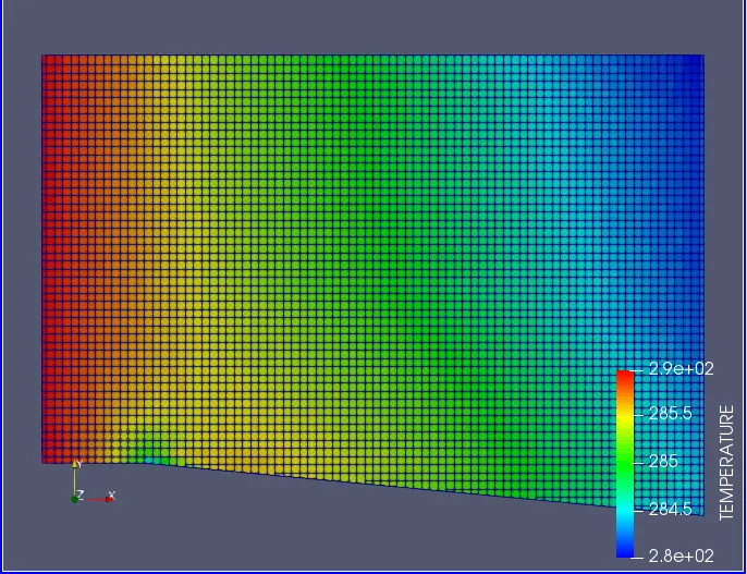
Figure 17: Final temperature contour during the subsonic flow simulation
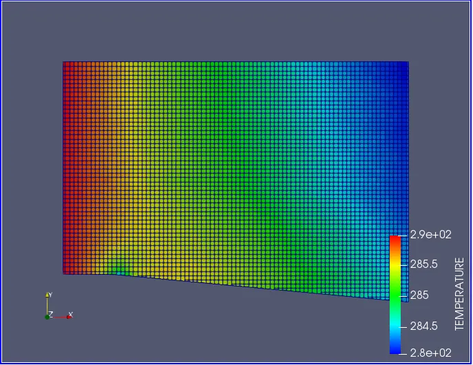
Figure 18: SGS of the subsonic flow
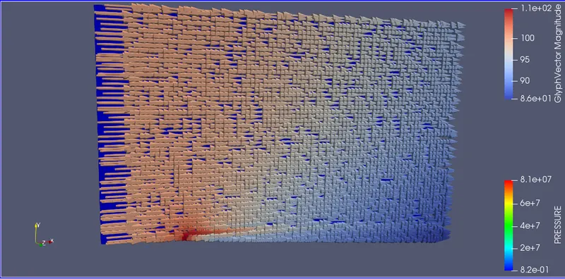
Figure 19: Vector gradient of the subsonic flow simulation
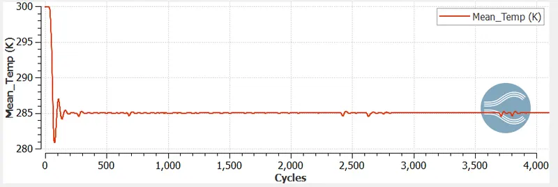
Figure 20: Mean temperature flow at subsonic flow simulation
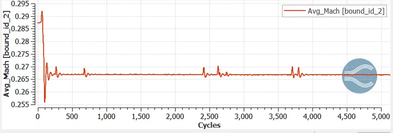
Figure 21: Average Mach number during the subsonic flow simulation
EXPLANATION: -
In that Prantyl Meyer shock flow problem, the main classification for that the flow has differed as supersonic flow and subsonic flow. In that each case SGS value is can be varied as 0.5 and 2.5. All four cases are should be derivate in this problem. In that first case using the Dirichlet boundary condition set as the pressure value is zero normal gradients and the velocity value is fixed as 680 m/s consider with the light velocity it high, where the Mach number of the flow is fixed as 2. The temperature value is set as 286.1K for the flow, For the outlet boundary condition is identified as Neumann boundary condition where the pressure value is zero normal gradients and velocity value is zero normal gradients and the specified value for the backflow conditions. This flow is named as a supersonic flow for the Prandtl Meyer shock wave problem.
In this same condition using the AMR, the SGS value is set as 2.5 for the first case and in the second case, it should be set as 0.5. For the two flows are supersonic flows, in that flow the differs the two SGS values. The flow creates the different types of SGS for the two cases.
The same condition follows the Inlet velocity is set as 100 m/s, its lesser value compare to the light velocity and the temperature is set as 281.6 K for the case 3 and the SGS differ for this subsonic problem also 2.5 and 0.5.
CONCLUSION: -
In this problem, different types of boundary conditions and SGS values are used to analyze the shock flow through the rectangular flow for the shock flow problem by using Converge 3.0.
Link for the video in YouTube: https://youtu.be/W0_oY0ocaeQ