Week 4.2: Project - Transient simulation of flow over a throttle body
Project - Transient simulation of flow over a throttle body
AIM:-
To set up and run the transient simulation of flow over a throttle body and find the pressure, velocity and mass flow over through the body by using the Converge 3.0 software.
INTRODUCTION: -
In this transient simulation flow through the pipe, the throttle wall surface is fixed as a rotating motion and surface movement is moving one. In this regard, the flow passing through the pipe the throttle rotates through the direction of the flow in the air. The flow of the air passing through the pipe whenever the throttle surface is open the velocity of the air also increases.
PROCEDURE: -
Step 1: Creating the 3D model of the throttle body elbow pipe using the modeling software in the format of .stl file.
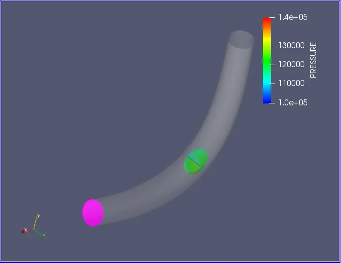
Figure 1: Transient flow over the throttle body
Step 2: Using the converge studio index open the .stl elbow pipe and add a single boundary.
Step 3: The wall thickness of the pipe should be neglected for this transient simulation process. To eliminate the thickness by using the geometry commands.
Step 4: Using the boundary command-click find separate the fence and select the boundary area and click the delete option.
Step 5: Next click the arc command select by angle delete the circular object. Then by using the diagnosis command find the open edges.
Step 6: Click the repair and patch option then select the open edges to click apply all the open edges are closed. Must verify the command by using the diagnosis command.
Step 7: Select the boundary command-click to add boundary 5 more boundaries are added.
Select the inlet and outlet boundaries are 1 and 2 respectively.
Step 8: Select the total elbow wall in boundary 4 named as elbow wall.
Step 9: Next to select the throttle valve, hide the elbow wall by using the box pick option, select the by surface method total throttle valve is selected as the boundary 3 from the body.
Step 10: After the separation of all boundaries click the setup option and click the Application type and select the time-based option, here the problem was a transient condition, it’s not an IC engine problem it depends on the time only.
Step 11: Next to select the materials, the predefined mixture was air and select the option as gas simulation, add the species option and select ok.
Step 12: Next for the global transportation parameters as the default option is selected and the species option-click and add the O2 and N2 are the airflow inlet gases.
Step 13: Next for the simulation parameters click the solver as a transient solver, it’s the necessary condition for this case. For the miscellaneous option select, the deselect the steady-state monitor option.
Step 14: Next for the important step, simulation time parameters set the start time is 0.0 Cycle, End time is 15000 cycles, Initial time step is 1e-7, Minimum time step is 1e-7 and the maximum time step is 1 second.
Step 15: Next for the solver parameters Navier – stokes solver type is pressure-based and pressure precondition is none and transient solver Initial PISO convergence criterion multiplier value is must below 1 set the value is 0.5.
Step 16: Next to select the boundary conditions for the flow as first for the inlet flow pressure is set to be 1.5e5 Pa and airflow also added.
Step 17: For the outlet select the pressure as 1e5 Pa and also added the air in the outlet flow. The elbow wall is selected as a wall boundary and it's selected as a no-slip wall.
Step 18: Deviation from the steady-state flow, the throttle surface is in the velocity boundary condition wall motion type is selected as rotating and the surface movement is set as moving and the center of rotation and rotation angle are identified.
Step 19: To hide all bodies without the throttle cylinder setup select the option measure and click direction continue with arc normal select the three different points using arc option and apply the center and about axis values are shown in the message log area, copy the values and add the boundary section axis center and about axis values.
Step 20: Rotation of the throttle is set as input file for 0.002 sections fixed as 250, that input file is named as throttle position.in and saved as the export file.
Step 21: For the base grid selection the grid value is set to be 0.002m for all the directions.
Step 22: In this grid selection also added an embedding selection, it’s very useful to separate the elements in the complicated shapes in an ahead manner. The fixed embedding creates the minimum size of the elements creations.
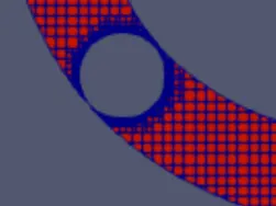
Figure 2. Fixed Embedding of the throttle wall
Step 23: Next for the post variable selection select the two species in the field of mass fraction and select ok.
Step 24: The time interval for the 3D output data files is 1000 Cycles and the Time interval for writing restarting output is 1000 cycles are should be selected in the field of post-processing selection.
Step 25: Finally export all the data into the selected folder and also copy the mpiexec and converge-intelmpi files into the folder and run the program.
Step 26: Also post-processing is done using the converge 3.0 simulation process .vtm group file also created.
RESULTS: -
Pressure and velocity contours for the transient flow over the throttle body
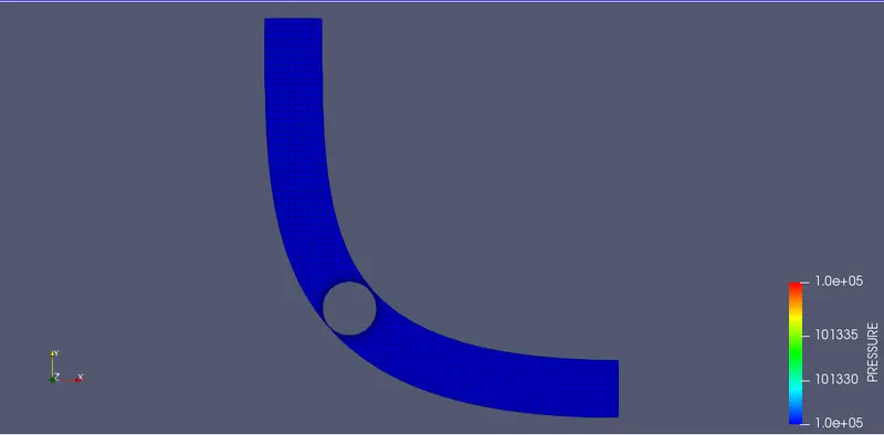
Figure 3. Mesh plot contour for the transient flow of throttle body
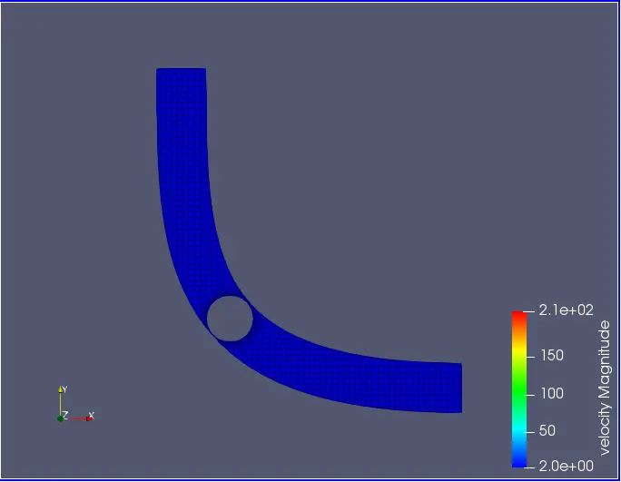
Figure 4: Initial velocity contour of the transient flow
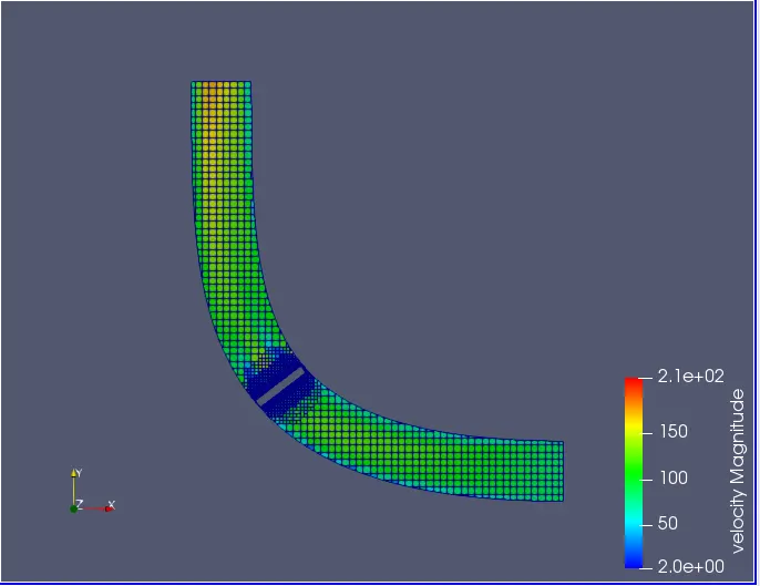
Figure 5. Final velocity contour for the transient flow
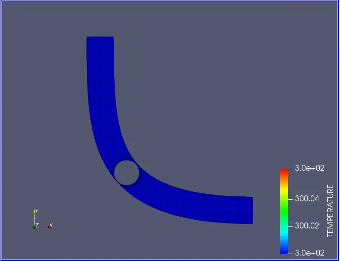
Figure 6: Initial temperature contour for the transient flow
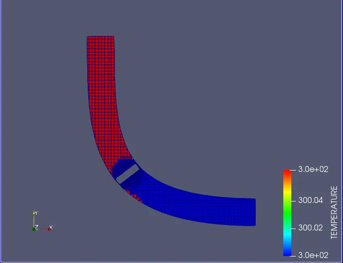
Figure 7: Final temperature contour in the transient flow before reached steady state
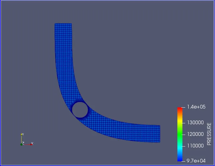
Figure 8: Initial pressure contour for the transient flow
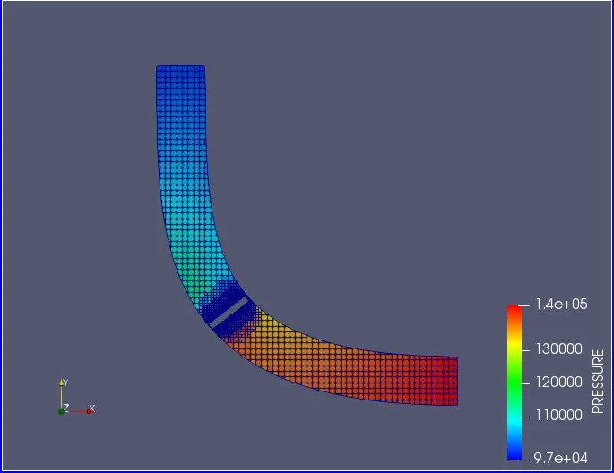
Figure 9: Final pressure contour in the transient flow over the throttle body
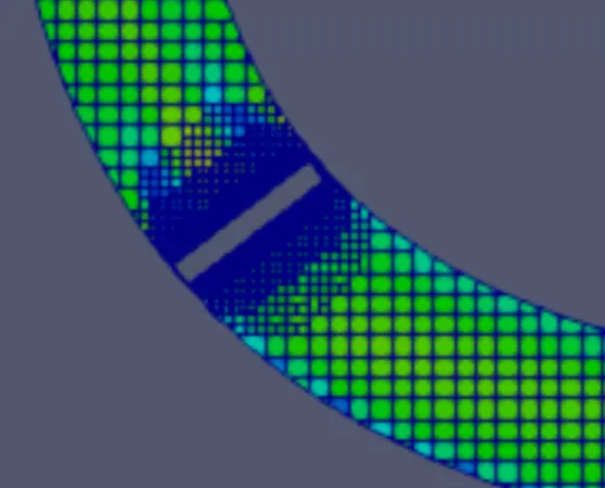
Figure 10: Throttle motion 2D during the transient simulation over the throttle body
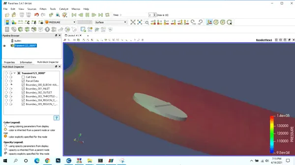
Figure 11: Throttle motion 3D during the transient simulation over the throttle body (GIF File)
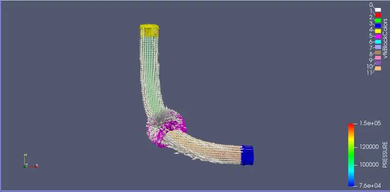
Figure 12: Pressure Vector plot contour of the transient flow over the throttle body
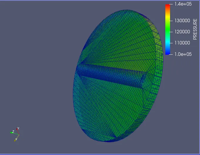
Figure 13: Throttle surface during the simulation with edges
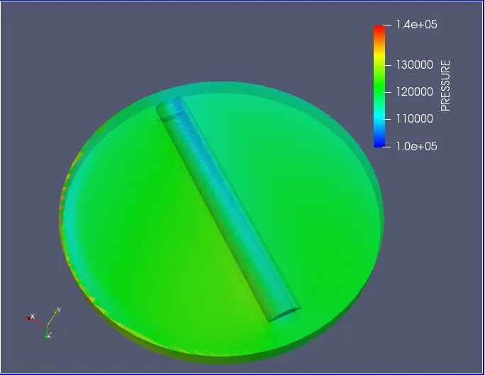
Figure 14: Throttle surface during the simulation without edges
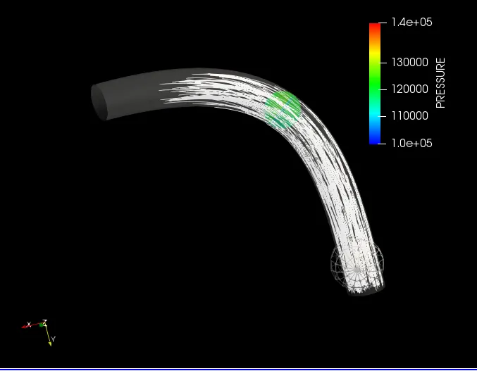
Figure 15: Steam tracer contour of the transient flow over the body
Mass flow rate of the transient flow through the throttle body
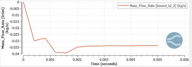
Figure 16: Inlet mass flow rate
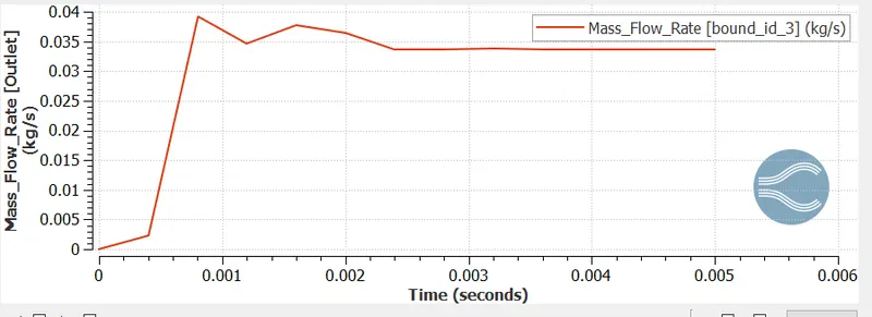
Figure 17: Outlet mass flow rate
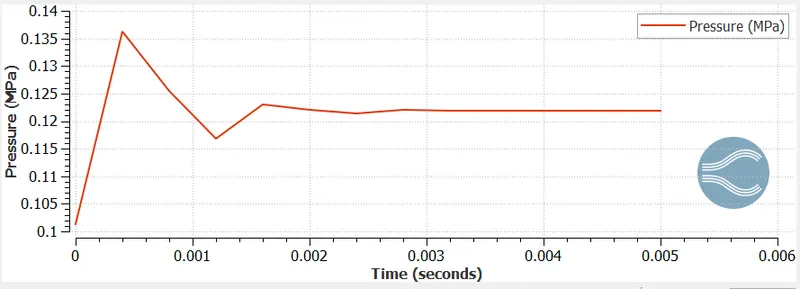
Figure 18: Pressure generation of the transient flow
Total cell count of the transient flow
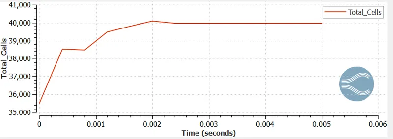
Figure 19: Cell count of the transient flow
Total cell count calculation: -
The average velocity of the transient flow is = 65 m/s
Minimum cell dimension = 0.4 m
End time calculation = minimum cell dim / Avg.Velocity = 0.4/65 = 0.005 s
For the total cell = 0.4/ 0.00001 = 40,000 cells
EXPLANATION: -
In the transient flow simulation, the total body is a fixed boundary except for the throttle surface. The throttle surface is set as a moved rotational object through the airflow through the pipe, the angle of the rotational surface is fixed as at 0.002 s the angle set as 25 degrees. The rotational throttle body position also selected as the input file. The input gives that whenever the throttle surface opens the velocity of the total pipe is increased. Then, when the air flows through the pipe the throttle body cylinder surface is getting the high pressure and the other surfaces only attained the minimum pressure. The pressure deviation mainly depends upon the angle of rotation of the throttle body.
CONCLUSION: -
The pressure and velocity variation over the throttle body were analyzed in the transient flow simulation process. The study of different regions formed showed that the throttle body and the velocity, temperature and pressure contour plots are analyzed using Converge 3.0 software.
Link for the YouTube Video: - https://youtu.be/POWaM2nNJDU