Week 6: Conjugate Heat Transfer Simulation

Aim: Conjugate heat transfer simulation using Converge Cfd and post processing the results.

Objectives:

• Setup a flow simulation through a pipe with inlet Reynolds number should be 7,000 for air.
• Add supercycling parameter asnd also Y+ in our post.in file.
• Simulate the results for different base grids for grid dependence test, and also for different supercyclying stage interval.
• Plot the results for all the cases.

Introduction:

CHT(Conjugate heat transfer):

We use conjugate heat transfer technique when heat transfer occurs simultaneously in between fluid and solid region.

The predominant mode of heat transfer in solid is conduction.

The predominant mode of heat transfer in fluid is convection.

The heat transfer is calculated using energy equation because we use 1st law of thermodynamic to derive energy equation which consist of heat term.

Heat transfer in solids:

Energy equation in solid side is given as:

where,

∇.(k∇T) = Heat flux due to conduction

Q = Volumetric heat source

Cp = specific heat

ρ = density(kg/m3)

Heat transfer in fluids:

Due to the fluid motion, three contributions to the heat equation are included:

1. The transport of fluid implies energy transport too, which appears in the heat equation as the convective contribution. Depending on the thermal properties on the fluid and on the flow regime, either the convective or the conductive heat transfer can dominate.
2. The viscous effects of the fluid flow produce fluid heating. This term is often neglected, nevertheless, its contribution is noticeable for fast flow in viscous fluids.
3. As soon as a fluid density is temperature-dependent, a pressure work term contributes to the heat equation. This accounts for the well-known effect that, for example, compressing air produces heat.

Accounting for these contributions, in addition to conduction, results in the following transient heat equation for the temperature field in a fluid:

Application:

(Engine heat transfer)

• Heat transfer from engine block to the coolant.
• Engine block heating due to conduction.
• Forced convection cooling of engine block.

CHT modeling setup:

• Defining the fluid and solid materials with physical properties.
• Configuring the fluid and solid regions.
• Assign regions to streams.
• Use appropriate boundary condition for the boundaries that separate different regions.
• Select time control methods.
• Set up the post processing.

Process steps(Supercycling workflow):

• In first we see that solver solves the solid, and fluid together with transient solver.
• After above process the heat transfer co-efficients, and temperature instantaneous values are stored.
• The fluid solver is stopped/freezed.
• Time averaged heat transfer co-efficient and temperature are applied as boundary condition for solid region and solid is solved using steady state solver until its convereged to a particular value
• Update the solid temperature field and unfreezes the fluid solver.
• Repeat above steps until solid and fluid temperature converges.

y+ and boundary layer:

boundary layer:

A boundary layer is a thin layer of viscous fluid close to the solid surface of a wall in contact with a moving stream in which (within its thickness δ) the flow velocity varies from zero at the wall (where the flow “sticks” to the wall because of its viscosity) up to U_e at the boundary.

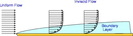
The boundary layer is layer where the velocity is approximately equal to 0.99 of free stream velocity.

u = 0.99 U

At the wall the velocity is zero(No-slip condition), and the velocity increases as a function of global cordinate y, there is gradient of velocity we can say this is due to shear stress acting upon the layer of free stream due to its viscosity, the shear stress above boundary layer is zero hence the velocity is equal to free stream velocity.

• The boundary layer thickness is greater for turbulent flow and lesser for laminar flow.
• We would like a measure of distance that scales with the boundary layer, because of which the y+(dimensionless quantity) was discovered.

Steps to calculate y+:

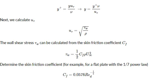
• Why we choose ut(frictional velocity) ?

Since the velocity at the wall is zero(No-slip), and also the free stream velocity can not be used inside the boundary layer which is the reason we use fricitional velocity.

• We can calculate the value of Cf if we know reynolds number and then can calculate y+ by using above formulas.
• y+ values are very important to guess whether our solution will give accurate values or not when combined with wall function.

Wall functions:

Wall function are the empirical function that are fitted to the observed behaviour closer to the wall.

• Why we need wall functions?

As we get near to wall the gradient(temperature,velocity etc) gets stepper, and in CFD simulators we generally use second order equation which is linear, because of linearity many numbers of cells are required to capture accurate value of certain parameters, this leads to very finer cells at wall hence high aspect ratio if there is skewness in cell it may lead to poor cell quality which will lead to divergence and instaility in the solution, hence in wall function we use non linear equation to accomodate the variation near the walls.

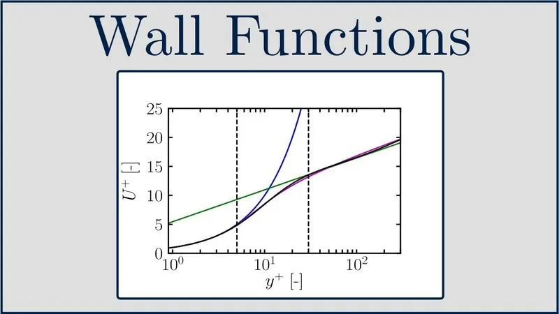
Experimental measurement of direct numerical simulation(DNS) close to the wall

• Now the above image shows the variation of y+(wall normal distance) and U+(dimensionless velocity) near the wall.

1. For y+ < 5 , blue line exactly fit the data (Sub viscous layer)
2. For y+ > 30 , green line exactly fit the data (log law layer)
3. For 5 < y+ <30 , is known as buffer region there is no curve to fit this data points.

• The standard wall functions can be given as:

1. U+ = y+ , y+ < 5 (linear)
2. U+ = (1/κ)*( log(E*y+)) (Logarithmic variation)

• κ and E are the empirical co-efficient.
• We have wall function values at sub-viscous layer and log law layer, but to calculate the value at buffer layer we can use simple logic.The wall functions intersects at y+ = 11.25

So the model for buffer region can be given as,

1. U+ = y+ , if y+ < 11.25
2. U+ = (1/κ)*( log(E*y+)) , if y+ > 11.25

• This procedure will lead to large error, hence general recommendation is to use the y+ values <5, and >30 for which we have wall functions defined.
• The alternative can be fit a single, smooth function through the entire range of y+, namely spalding's wall function.

y+= (U+) + E*[exp(κ*U+)−1−(κ*U+)−0.5(κ*U+)2−16(κ*U+)3] , valid for y+<300

Converge CFD simulation setup:

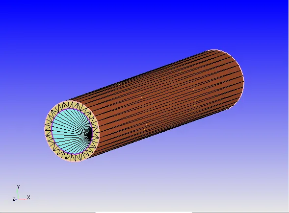
Creating a geometry and running a diagnosis to fine errors the error we see is non-manifold edges which will be resolved once we finish the case setup.

Case set-up tree:

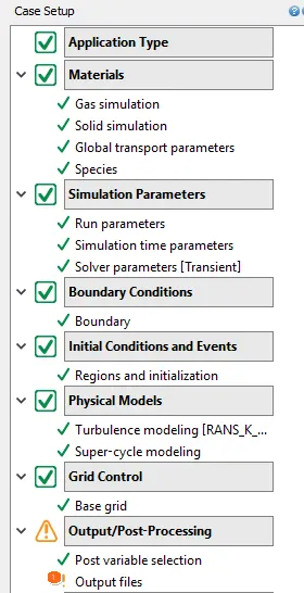
Materials:

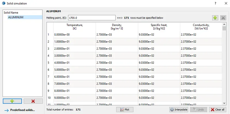
• In solid simulation we should select a predifined solid and its properties varying with temperature(we select aluminium as our solid)
• In species we will add(O2,N2) for gas, and(AL) for solid and validate.

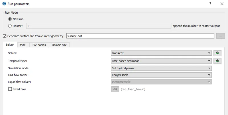
Simulation parameters:

• In run parameters we will set simulation for transient flow case.

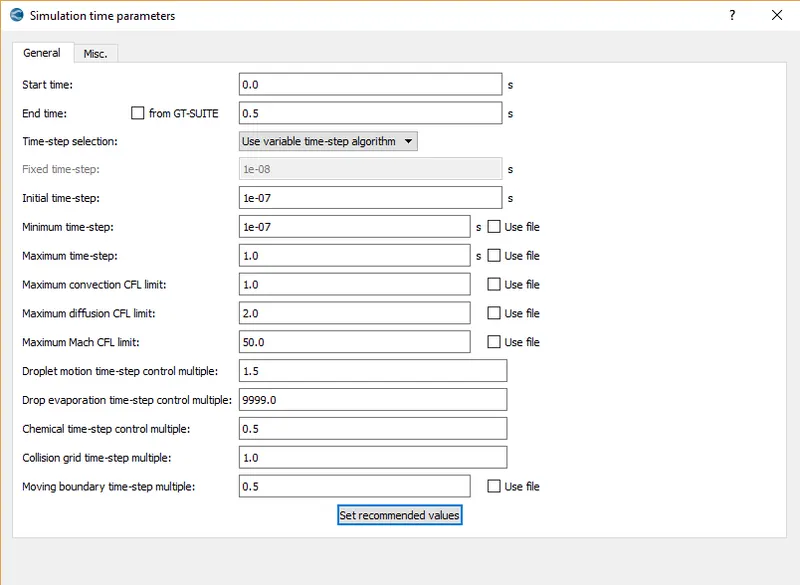
• Simulation time parameters are given as,

Boundary:

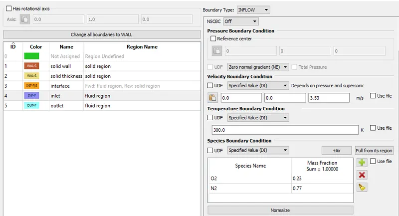
Inlet:

• Boundary type: Inflow
• dirchilet bounadry condition with specified velocity.
• Velocity is calculated based on reynold's number which is given as 7000.

Re = (rho*V*D)/(Dynamic viscosity)

Given,

rho = 1.225 kg/m3

Dynamic viscosity = 1.844*e-5 kg/m.s

D = 0.03m

V = 3.53 m/s

Interface boundary condition:

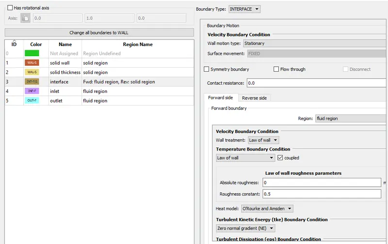
• If there are two different phases the interface boundary condition is applied to separate two phases.
• The interface boundary codition consists of reverse coupling and forward coupling.
• In case of the pipe with interface boundary if normals are facing towards inwards it is our fluid domain and forward coupling region, and reverse coupling region is solid.
• The coupling between two materials/phases can be of two types namely,

1. Contact resistance = 0 : temperature is continous at the boundary.
2. Contact resistance > 0 : temperature is discontinous at the boundary.

• When two surface are coarse enough that there is gap inbetween when the are attached together we can find that inbetween the solid surface the fluid/air is been trapped which causes the contact resistance in solids. In case of fine surface we can neglect the contact resistant in solids.
• In fluids ,and solids interface the contact resistance is generally due to a insulation in between a surface, e.g. thermal barrier coating.

Wall boundary:

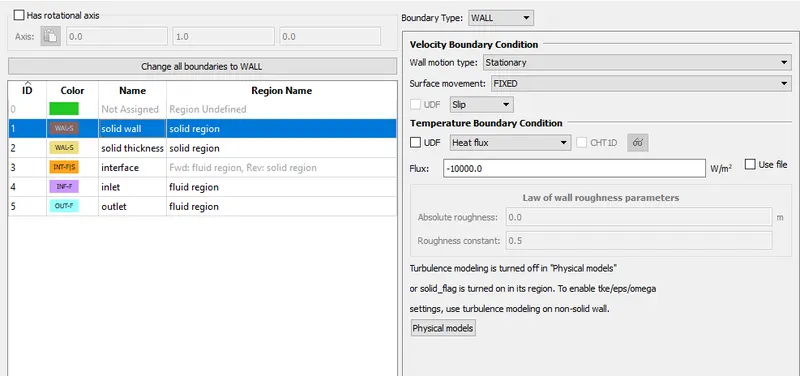
The possible wall boundary condition for temperature specification are:

Dirichlet boundary condition:

In which we specify the values at boundary directly.

Heat flux :

In which we specify heat flux entering or leaving the system.

Convection :

In which we specify far field temperature and value for heat transfer co-efficient(Hconv).

• In our simulation we specify the heat flux boundary condition with (flux:-10000W/m3)

Solid thickness(wall):

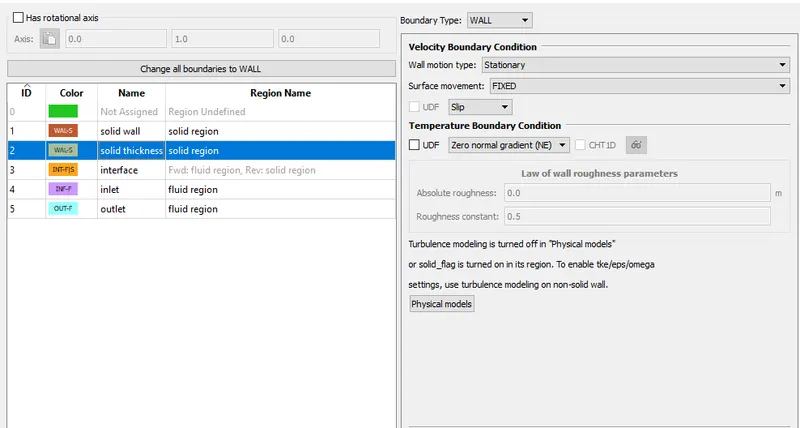
• Slip and adiabatic(No heat transfer) conditions are applied.

Regions:

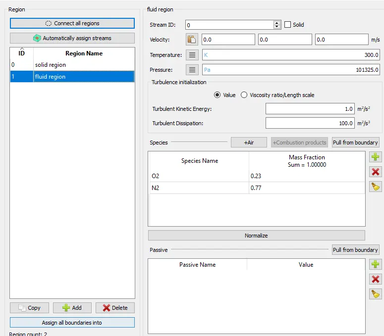
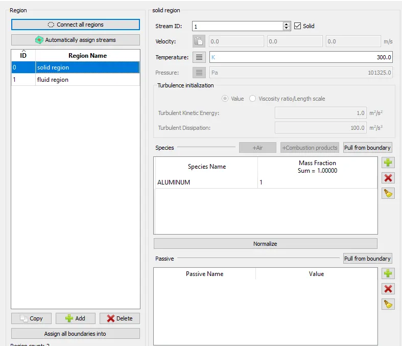
Two region are specied solid region, and fluid region.

Stream:

• A stream is collection of connected regions of the same phase.(solid,liquid etc)
• If we have two different phase such as solid and liquid the stream id for them should be different since we are solving different set of equation for both the cases.
• We can apply same stream id for multiple regions in same phase if all the regions are connected to each other.
• Converge stream specifications:

1. Stream ID = 0 for fluids
2. Stream ID = 1 for static solids
3. Stream ID > 1 for moving solids

• The Stream ID for moving solids are same if they have same motion profile or it must be different for all the cases.

Supercycling process:

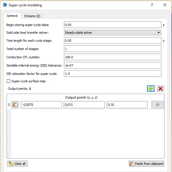
• Supercycling is package which is used by Converge to solve conjugate heat transfer problems.
• The reason for using this method is both the solver cannot run at same speed. The fluid side converges more faster then the solid, hence there should be a method in which we can control there speed.
• The basic idea behind the Super cycling is the fluid side solver is paused until solid side solution converges and once converged its unpaused and same process is repeated.
• Solid side heat transfer solver don't have any relation with run parameter.
• Time rate for each cycle stage defines the time for which the fluid is freezed until solid side solution converges.
• Output points is a point in solid region such that solver can get the values at solid to verify whether solution is converged or not.

Post variable selction:

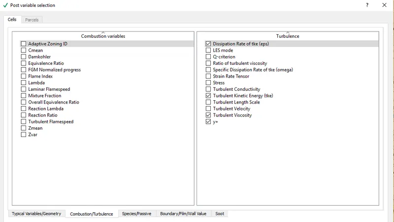
• The only change in post variable selction is we add y+ in our post.in file.

RESULTS:

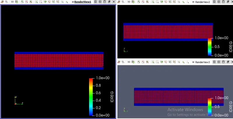
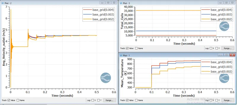
Conjugate heat transfer simulation for different base grid sizes(0.004,0.003,0.002):

Mesh for all base grids defined by registered stream ID's:

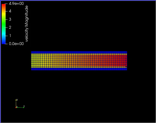
Velocity contours:

Velocity contour for base grid size(0.004m):

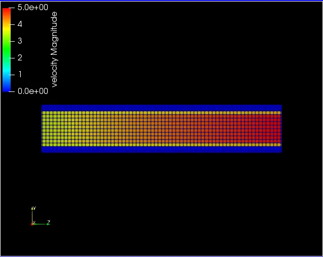
Velocity contour for base grid size(0.003m):

Velocity contour for base grid size(0.002m):

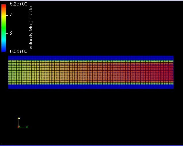
As the base grid size increases we get more accurate value for velocity which can be compared from legends of different velocity contours.

Y-PLUS contours:

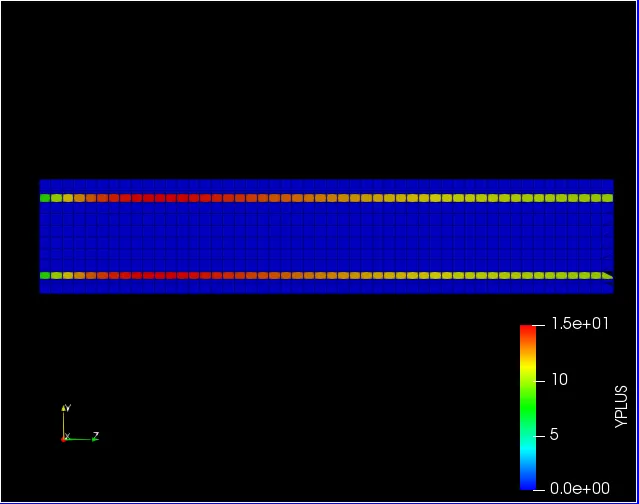
Y-PLUS for base grid size(0.004):

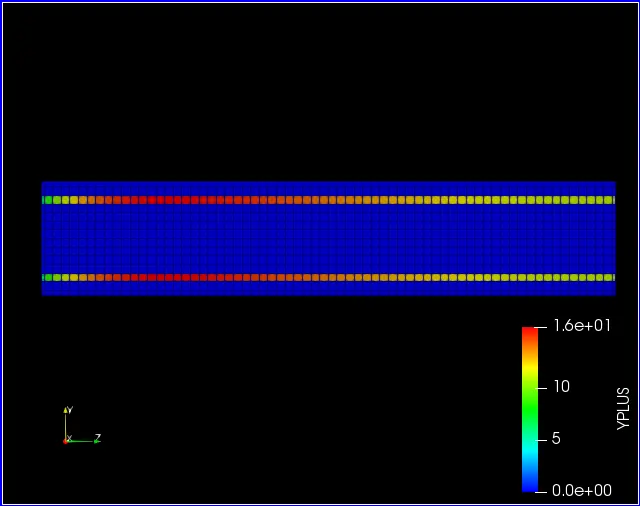
Y-PLUS for base grid size(0.003):

Y-PLUS for base grid size(0.002):

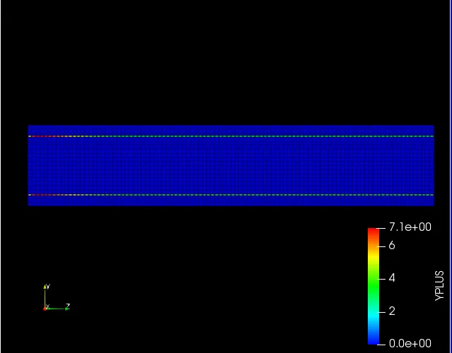
As we can see from the plots that normal distance for different grid size decreases and less for fineer meshes, less y+ value is good because it gives a accurate solution which we have discussed in theory part.

Glyph:

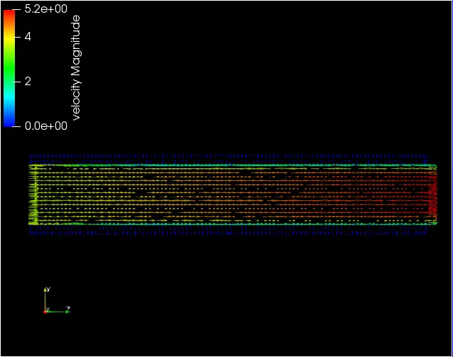
Shows the direction of the flow.

Plots for average velocity, total cell count, and mean temperature for different mesh sizes:

Conjugate heat transfer simulation for different cycle stage value(Supercycling) and base grid 0.004m:

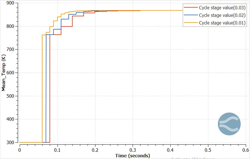
As we decrease the cycle stage value the solution gets converged soon. since smaller cycle stage time means the steady state solver starts its work before which will lead to fast convergence.

Video link:

https://drive.google.com/file/d/1_EOebAVUSSTWsD3519xe4SLDc-4N1tM6/view?usp=sharing