Week 6: Conjugate Heat Transfer Simulation

1. AIM

Our aim is to setup a transient state conjugate heat transfer simulation of flow through a pipe in converge by using different stage interval for super cycling model and different grid size, simulate it using Cygwin terminal and post process in Paraview and check the results.

2. THEORY/EQUATIONS/FORMULAE USED

Structure of CONVERGE CFD simulations

The basic steps for a simulation are as follows,

1. Pre-processing [Converge Studio v3.0] – It is a leading CFD package for simulating 3D fluid flow. It is a user friendly interface which provides high productivity and easy-to-use workflows. Its features includes autonomous meshing, state of the art physical models, robust chemistry solver, and the ability easily accommodate complex moving geometries.
2. Solving [Cygwin] – It is a large collection of GNU and Open Source tools which provide functionality similar to a Linux distribution on Windows.
3. Post-processing [ParaView 5.9.0] – It includes analyzing the results by plotting the results as charts, contour, and exporting the data, also validating the results both qualitatively and quantitatively.

Conjugate Heat Transfer

Conjugate heat transfer is a combination of conduction and convection. It’s a heat transfer which involves the interaction of conduction within a solid body and convection between the solid surface and fluid volumes.

Typical example is a heat exchanger as in the figure the cold fluid enters the tubes and takes heat from the hot air flowing around the tube via natural convection. Some of the applications which involve conjugate heat transfers are building roofs, open water, chimney etc.

Heat Transfer Coefficient (HTC)

It’s a measure of convective heat transfer between fluid volume and solid medium around which the fluid flows.

Heat transfer coefficient is defined by the newton’s law of cooling. It is proportionality constant between heat flux (q) and temperature difference (ΔT) between the solid medium and the surrounding fluid. The SI unit of heat transfer coefficient (HTC) is watts per square meter kelvin (W/m²K).

For convective heat transfer coefficient calculation, usually T₂ is temperature of the solid surface and T₁ is temperature of the fluid around the surface or we can also call it as reference temperature. The choice of reference/ fluid temperature is important as the temperature near and away from the wall would be different depending on the flow due to thermal boundary layer.

There are two heat transfer coefficient for a flow through a pipe i.e. Internal HTC and External HTC

For External flows, fluid temperature will be the free stream temperature.

For Internal flow, fluid temperature will be the mass flow average temperature as the temperature profile inside a tube will be parabolic.

Nusselt Number

It is the ratio of convective heat transfer to the fluid heat conduction heat transfer under the same conditions.

Nu = qconvection /qconduction

Concept of Wall Function

Wall function is an important defining criterion that tells the solver about the approach to solve near the boundary wall as it’s different for every case.

The boundary wall may be laminar or turbulent as well.

1. For laminar boundary, wall will be in no-slip condition.
2. For turbulent boundary, the laminar region near the wall is very small.

There are three regions in the turbulent boundary layer.

1. Turbulent Layer [ 30 < Y+ < 300 ]
2. Buffer Layer [ 5 < Y+ < 30 ]
3. Viscous-sub Layer [ Y+ < 5]

Y+ value

Y+ value is used to determine the first cell height based on whether to use wall function or not. Wall functions are required as the gradients of velocity, temperature, etc. close to the wall are large.

There are two approaches for solving i.e,

1. Piecewise linear [Near Wall Approach] – where fine grids are required to accurately resolve the gradient near the wall.
2. Non-linear [Wall Function Approach] – where the first grid height is more and the viscosity affected area is skipped.

Super Cycling Modelling

Super Cycling Modelling used for Conjugate heat transfer problems where the equations need to be solved for both solid and fluid domains. This method is used in converge studio. Heat transfer occurs at a different speed in both solid and fluid domains as the convergence is achieved faster that the solid domain. So it creates a problem during solution as the convergence for both domains can’t be achieved at same time. In order to address this issue the super cycling model is used which makes sure that the equations are solved and convergence is achieved at the same time by pausing fluid domain solver until the solid domain are solved using time lengths for each intervals.

Problem – Flow through a pipe

The challenge includes transient state simulation of flow through a pipe, and to check the results.

Mesh Size - dx = dy = dz = 0.004 m [Base Grid],

dx = dy = dz = 0.003 m [Case 1],

dx = dy = dz = 0.002 m [Case 2]

Calculation

Inlet Velocity

Reynolds Number, Re = 7000, Density of air, ρ = 1.177 kg/m³ [for 300 K]

Diameter of the pipe, d = 0.03 m [Inner Dia], Dynamic Viscosity, µ = 1.86e-5 [for 300 K]

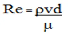
So, Inlet Velocity, v = 3.7 m/s

Total simulation time

Length of the pipe = 0.2 m, Inlet Velocity = 3.7 m/s [Reynolds Number = 7000]

Total Time required for single flow cycle = 0.2/3.7 = 0.05 [Time = Distance/ Speed]

Total Time required for 10 flow cycle = 0.05*10 = 0.5

So, End time taken, t = 0.5 s

3. PROCEDURE

• Firstly all the softwares are downloaded and installed in the system.
• Geometry is created in converge studio, boundary is flagged, and boundaries are checked for normals and orientation is done as per the requirement and finally diagnosis check is carried out to check for any errors such as intersections, open edges, overlapping triangles etc.
• In the heat transfer problem usually interface is present and it causes non-manifold edges, so it is ignored while error diagnosing as it will be taken care of while defining the boundary as interface.
• Case setup is done using setup wizard, then the input files are exported to a specific directory and also converge executable application are also copied into the directory.
• The simulation is run using Cygwin commands and post converted the output files so that it is compatible for post processing in Paraview.

4. NUMERICAL ANALYSIS
   • Geometric Model

The geometry of pipe is created and boundary is flagged as per the fluid and solid domain in Converge Studio as per the figure given below.

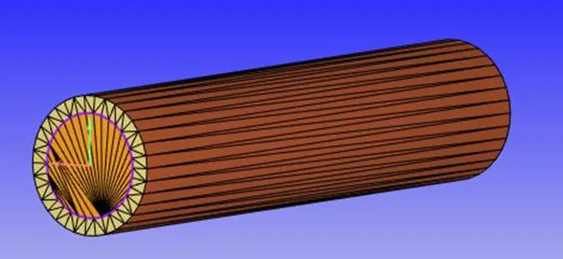
Fig: 3D Geometry – Pipe Flow

• Mesh

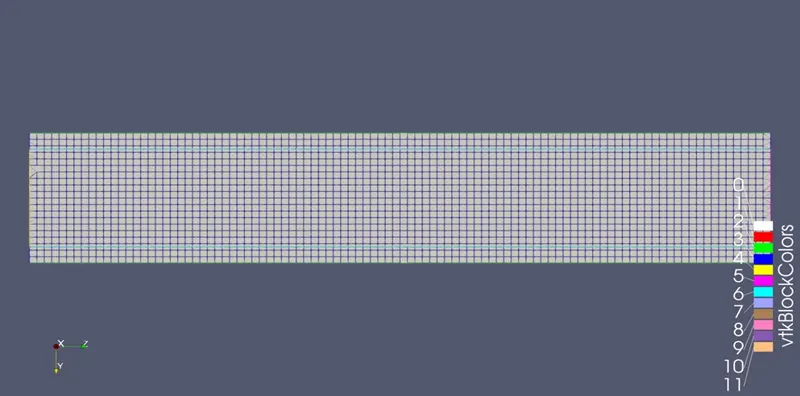
Fig: Mesh

• Boundaries

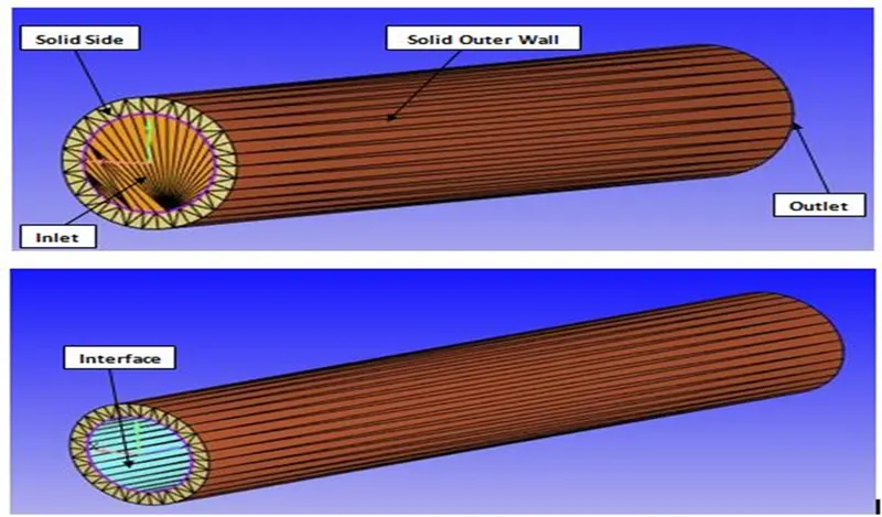
Fig: Boundaries of the domain

• Case Set-up

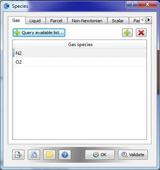
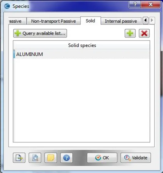
1. In Materials tab, materials – Air, species – O2, N2 [Fluid], Aluminum [Solid] and global transport parameters are selected.

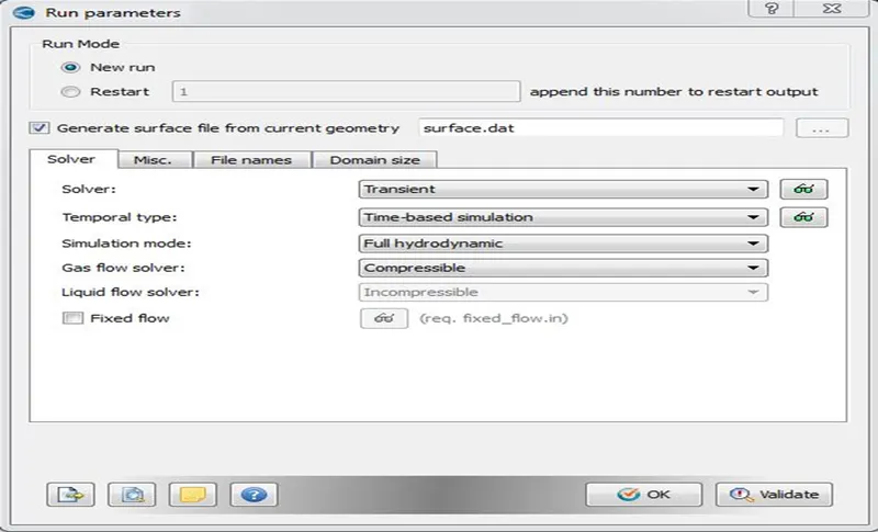
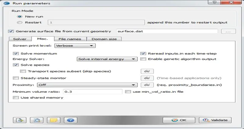
2. In Simulation Parameters tab, Run parameters such as Solver type, Simulation Mode and Gas flow Solver are set. In Misc. Tab uncheck the shared memory and steady state monitor.

3. Simulation time parameters such as total number of cycles, time step, CFL limits etc are set as shown in the figure below.

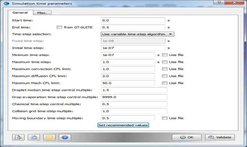
4. Solver parameters such as the Navier stokes solver type, equations preconditions type, solver controls are set.

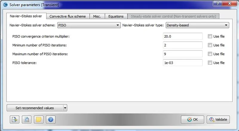
5. Boundary Conditions and Initial Conditions

Zone	Type	Boundary Condition	Additional conditions (if any)
Inlet	Velocity Inlet	Velocity Inlet – 3.7 m/s	Transient State, Density Based, Temp – 300 K Turbulence Model- Standard k-epsilon
Outlet	Pressure - Outlet	Static Pressure – 101325 Pa
Solid Outer Wall	Wall - Slip	Heat Flux = -10000 W/m2
Solid Side	Wall - Slip	Zero Normal Gradient
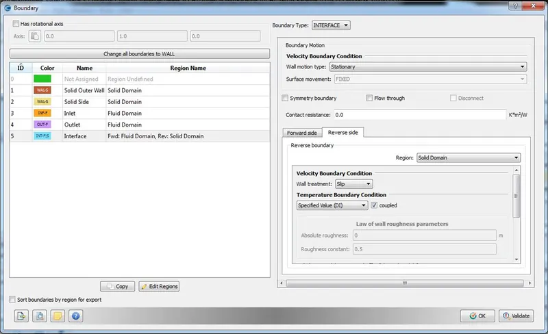
Interface	Interface	Forward – Fluid Domain Rearward – Solid Domain

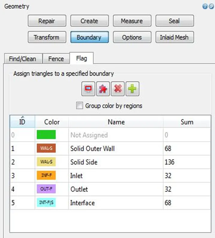
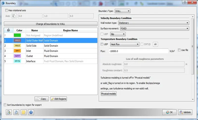
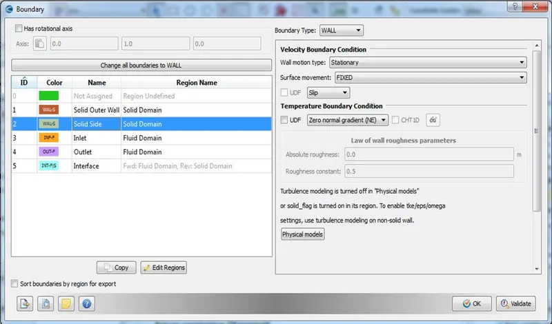
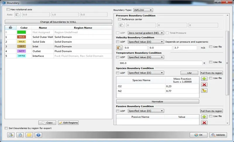
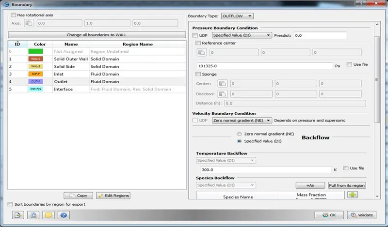
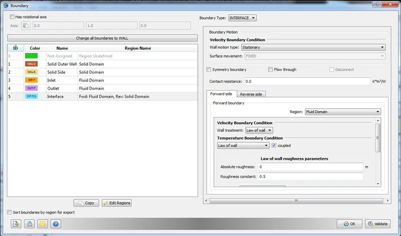
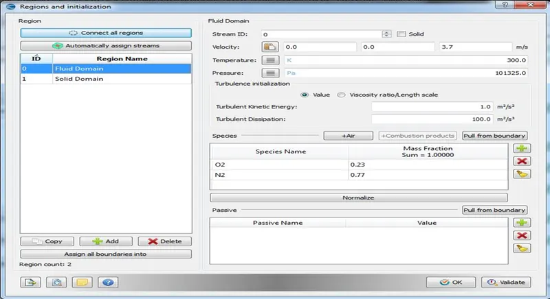
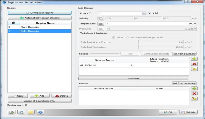
6. Regions and Initialization – Fluid domain is created and air is added as species with Stream ID as 0. Solid Domain is created and aluminum is added with Stream ID as 1.

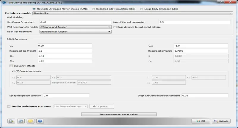
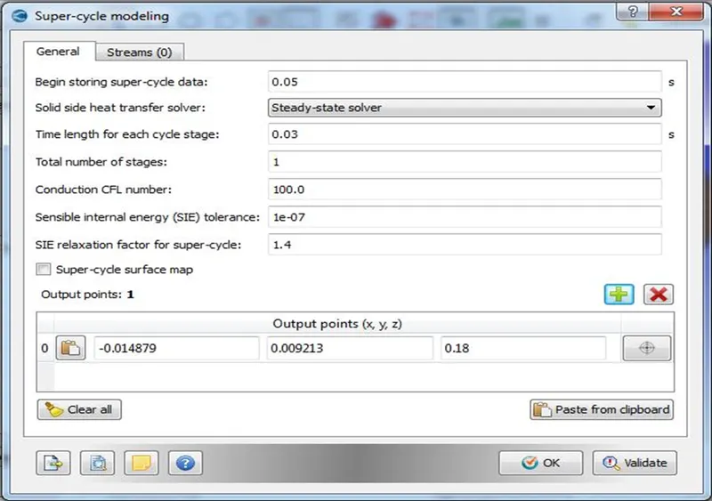
7. Turbulence Modelling – Reynolds Averaged Navier Stokes – Standard K-epsilon Model and Super Cycle Modelling done for Solid Domain with a monitor point being added.

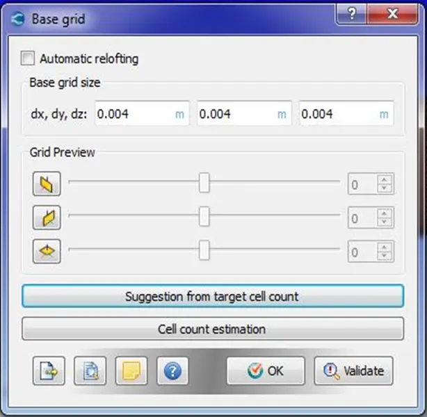
8. Base Grid – Mesh sizes are entered as per the problem.

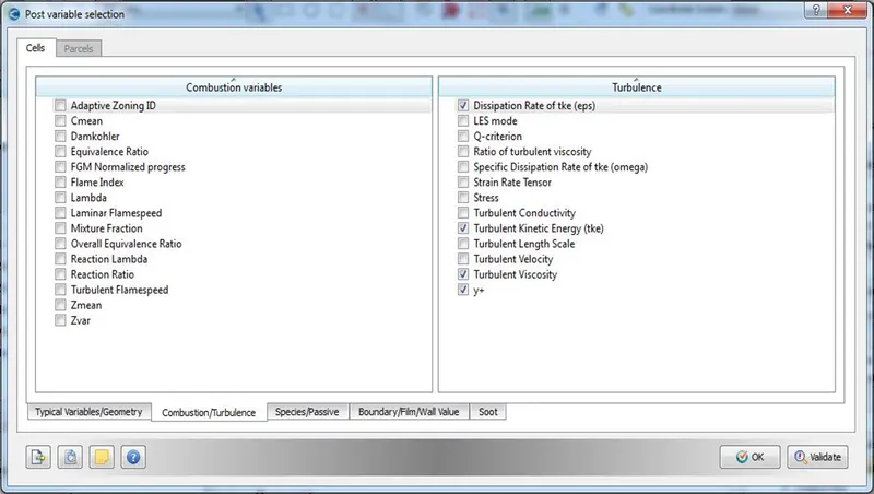
9. Post Variable Selection - Select all the necessary variables and the location that needs to be checked while post processing.

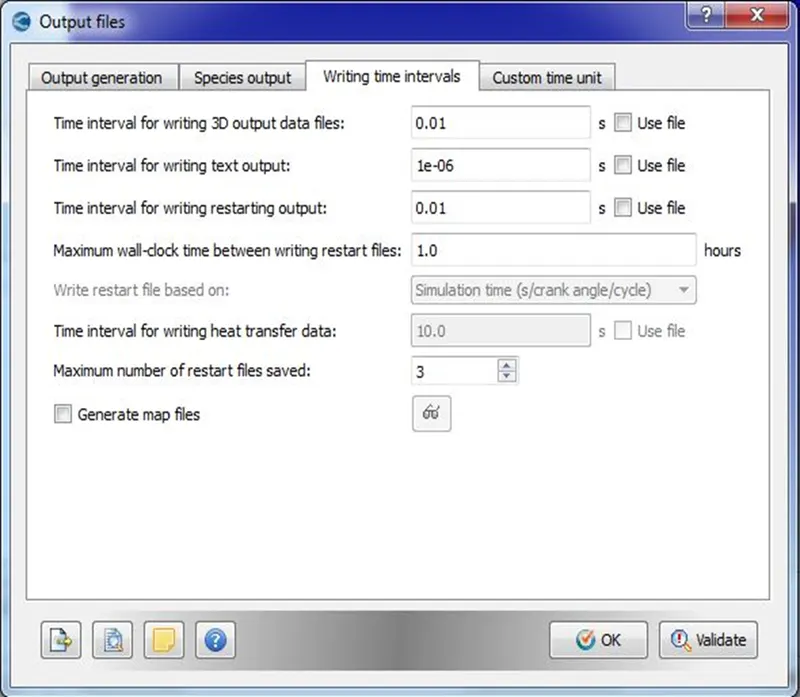
10. Output Files – Output files writing time intervals, restart files are set as per the requirement.

11. After the setup is done click on “Validate all” option to check for any issues with the case setup. If everything is correct then green tick will appear for all tabs as shown in the figure below. Once the Setup is done, export the input files.

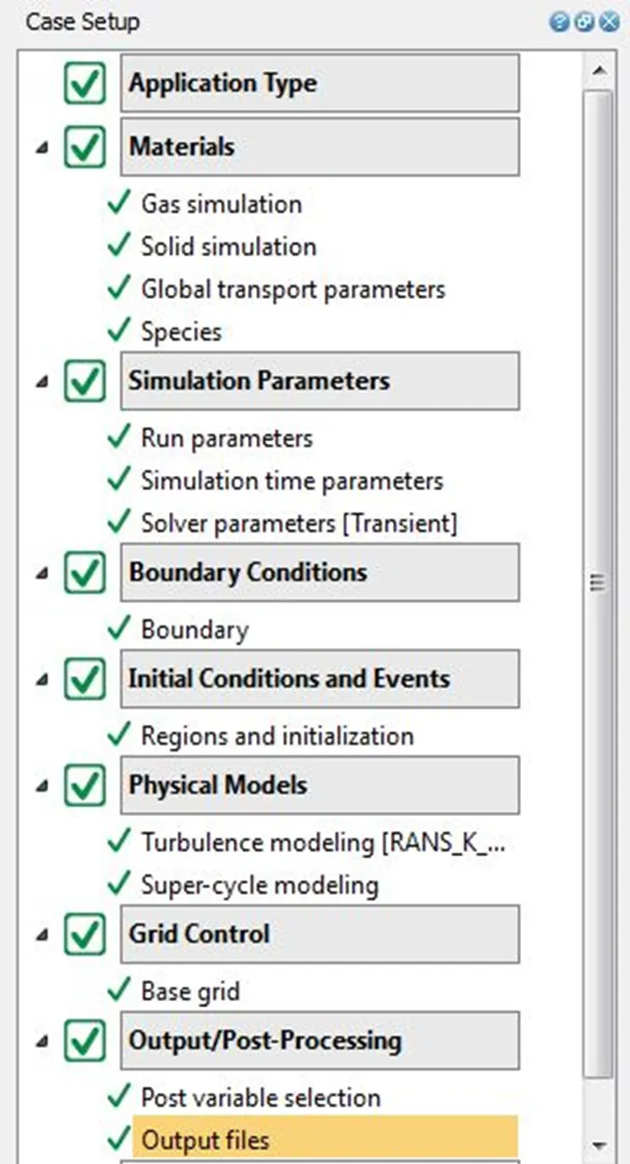
12. With input and executable files, navigate to the specific directory in Cygwin and run the simulation using "exe -n 4 converge.exe restricted </dev/null> logfile &"

13. After the run is completed Post convert the output files using “exe -n 4 post_convert.exe” into binary inline vtk format.

14. Using the vtm group files, post processing is done in ParaView in order to study the results.

5. RESULTS

Case Baseline (Inlet Velocity – 3.7 m/s, Base grid – 0.004 m)

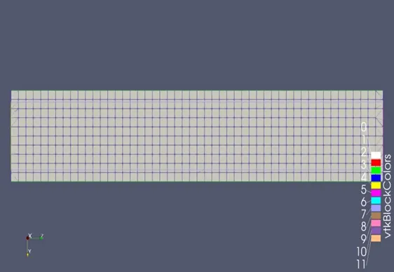
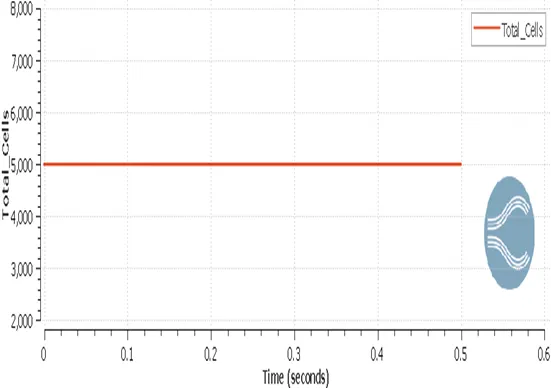
Fig: Mesh Fig: Total Cell Count

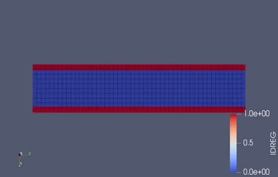
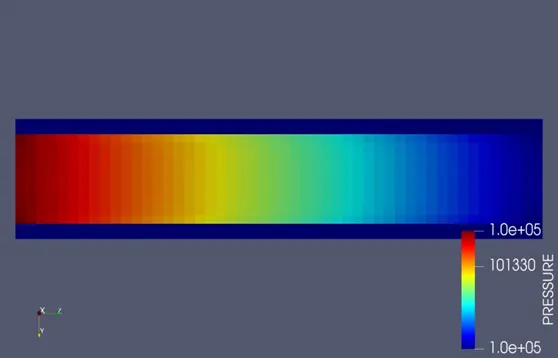
Fig: IDREG Fig: Pressure Contour

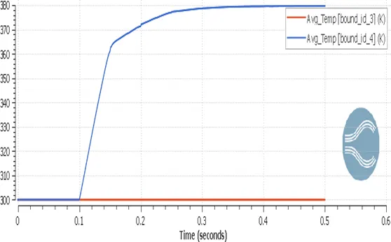
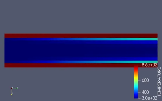
Fig: Average Temperature Plot Fig: Temperature Contour

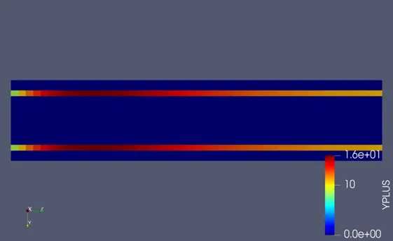
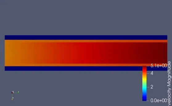
Fig: Y plus Contour Fig: Velocity Contour

Animation Link

Temperature – https://youtu.be/cwWGjTacZKY

Case 1 (Inlet Velocity – 3.7 m/s, Base grid – 0.003 m)

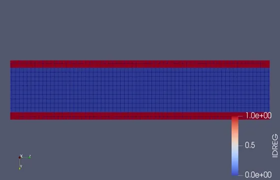
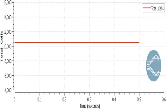
Fig: Mesh Fig: Total Cell Count

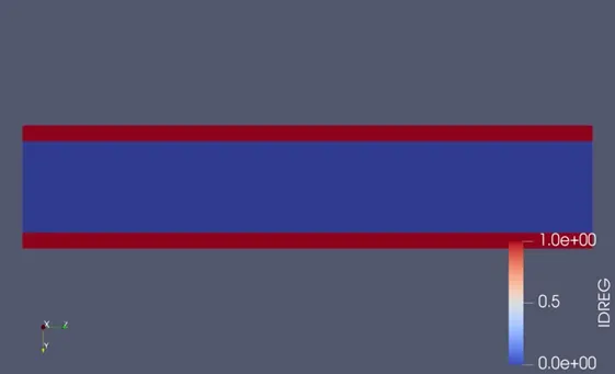
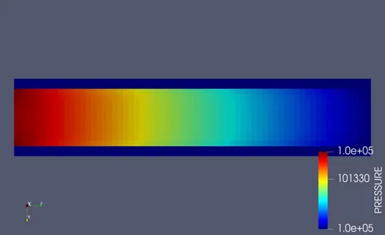
Fig: IDREG Fig: Pressure Contour

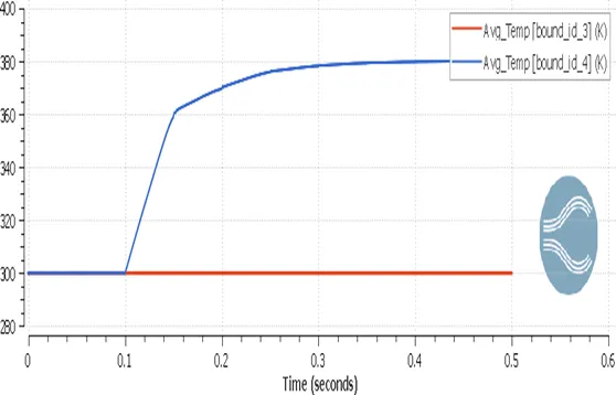
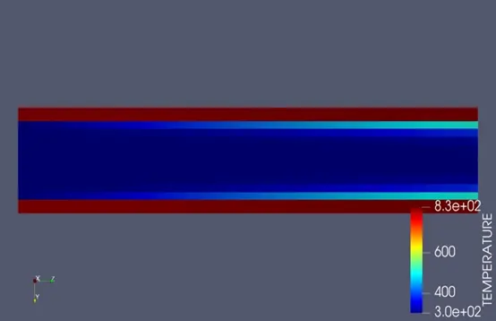
Fig: Average Temperature Plot Fig: Temperature Contour

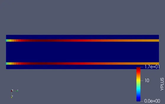
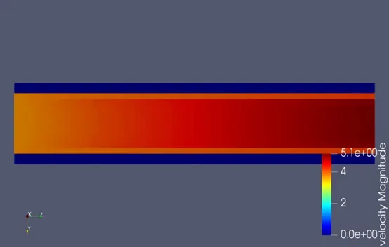
Fig: Y plus Contour Fig: Velocity Contour

Animation Link

Temperature – https://youtu.be/EhOhkB_rMPY

Case 2 (Inlet Velocity – 3.7 m/s, Base grid – 0.002 m)

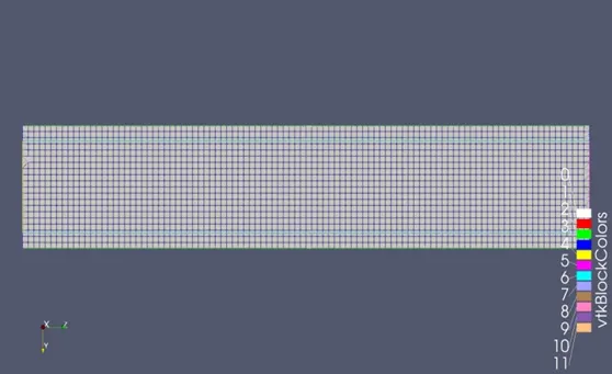
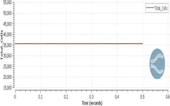
Fig: Mesh Fig: Total Cell Count

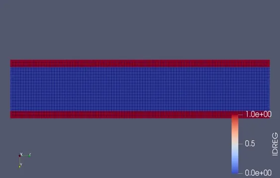
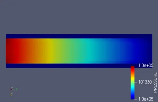
Fig: IDREG Fig: Pressure Contour

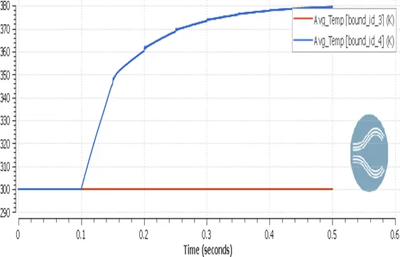
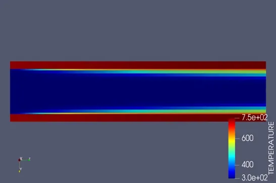
Fig: Average Temperature Plot Fig: Temperature Contour

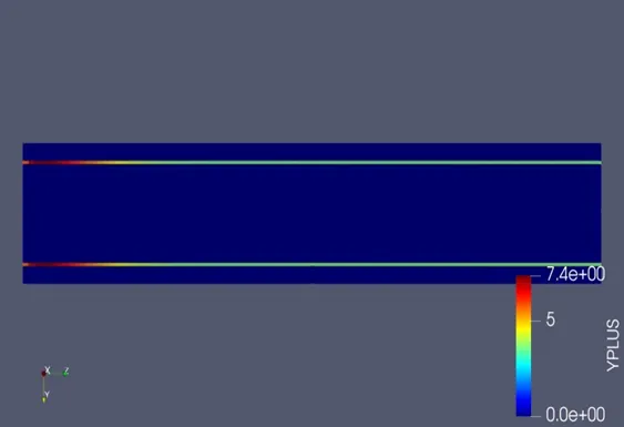
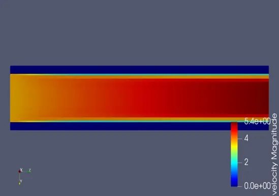
Fig: Y plus Contour Fig: Velocity Contour

Animation Link

Temperature - https://youtu.be/DzTDBrk8suw

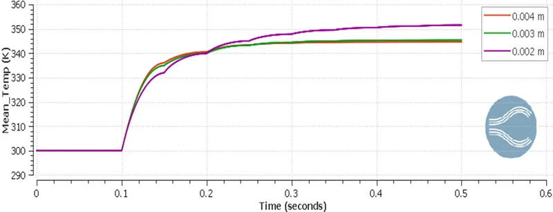
Fig: Mean Temp of Fluid Region

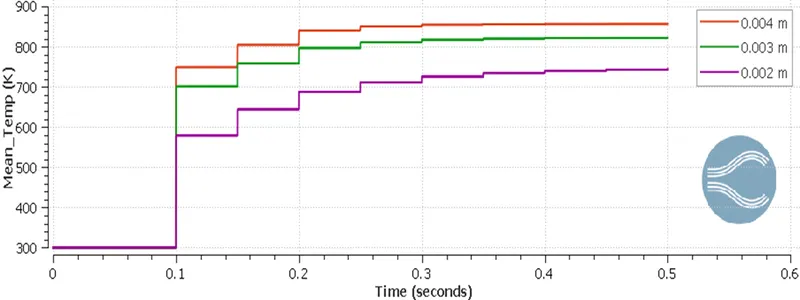
Fig: Mean Temp of Solid Region

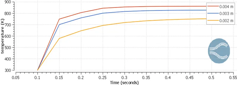
Fig: Mean Temp at the Monitoring Point

Super Cycling Modelling (Inlet Velocity – 3.7 m/s, Base grid – 0.003 m)

Case 1A - Stage Interval – 0.03

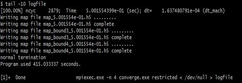
Fig: Simulation Time for Stage Interval – 0.03

Case 1B - Stage Interval – 0.02

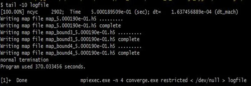
Fig: Simulation Time for Stage Interval – 0.02

Case 1C - Stage Interval – 0.01

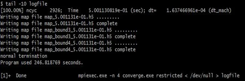
Fig: Simulation Time for Stage Interval – 0.01

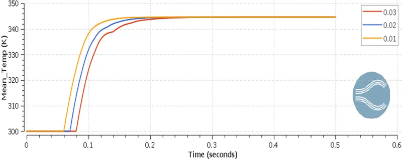
Fig: Mean Temp of Fluid Region

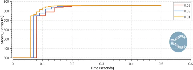
Fig: Mean Temp of Solid Region

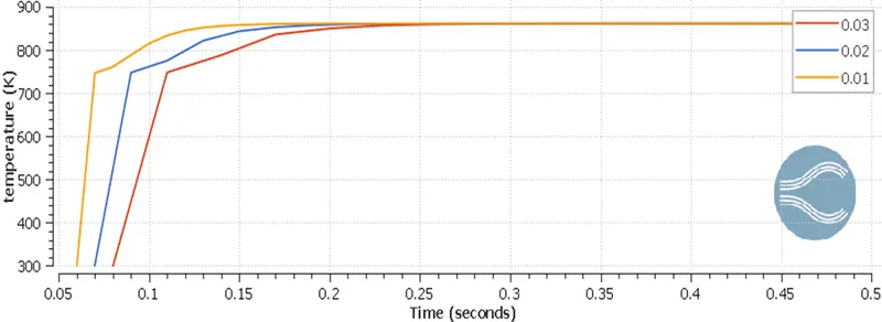
Fig: Mean Temp at the Monitoring Point

6. CONCLUSION

• Transient conjugate heats transfer simulation of flow through a pipe is carried out for 0.5 seconds.
• The heat flux of 10000 W/m2 is applied on the solid outer wall and inlet velocity is calculated as 3.7 m/s based on the given Reynolds number 7000.
• Cut cell meshing strategy is used in converge studio. The total cell count for baseline, case 1 and case 2 are 5000, 10500, and 36000 respectively.
• Solid and Fluid Domain of the pipe flow can be confirmed from the IDREG contour which shows the stream ID given while setting up the case.
• Contour shows that the pressure is high at the inlet and gradually reduces at the outlet to the specified in the outlet boundary conditions.
• Temperature contour and plot shows that the solid domain with different grid size of 0.004, 0.003 m, and 0.002 m attains different average temperature of 850 K, 820 K, and 750 K respectively. This can be confirmed by the temperature plot of the monitoring point in the solid domain as well.
• Temperature contour and plot shows that the fluid domain with different grid size of 0.004, 0.003 m, and 0.002 m attains an average temperature of 380 K at the outlet boundary in all cases.
• Contour also shows that the Y plus value reduces as the mesh becomes denser. Baseline and Case 1 has a max Y plus value around 160-170 but for case 2 the max Y plus value is 7.4. Due to this Case 2 shows the temperature of fluid near the wall even precisely.
• Super Cycle Modelling is done for case 1 with grid size as 0.003 m and stage interval as 0.03, 0.02, and 0.01 respectively. Results show that as we reduce the stage interval value the simulation time also reduces.
• Mean Temperature value of the fluid and solid domain converges at 345 K and 850K respectively for all 3 cases of stage intervals. It can also be seen that mean temperature for the solid domain converges faster with stage interval of 0.01 at 0.15s compared to stage interval of 0.02 and 0.03 at 0.19s and 0.23s respectively.
• The animation shows the temperature variation of the fluid domain due to the applied heat flux on the solid outer wall for three different cases with different grid sizes.
• The simulation correctly captures the physics of conjugate heat transfer clearly as it shows the heat flux applied on the solid outer wall transfers through the solid domain via conduction and then to the fluid domain via convection.