Week 6: Conjugate Heat Transfer Simulation
Conjugate Heat Transfer Simulation using Converge CFD
Aim: Setting up the airflow through the Aluminum pipe & Simulating the Conjugate Heat Transfer analysis between solid and fluid using Converge CFD.
Objectives:
- Grid dependence test:
- We have to perform a Grid dependence test on 3 grids and show that the outlet temperature converges to a particular value.
- Effect of supercycle stage interval:
- Set supercycle stage interval to 0.01,0.02 and 0.03. For these three values, how does the total simulation time compare against the baseline configuration
CHT analysis:-
The Conjugate Heat Transfer (CHT) analysis type allows for the simulation of heat transfer between solid and fluid domains by exchanging thermal energy at the interfaces between them.
- Simply, When the heat transfer occurs simultaneously within and between fluid and solid regions then it is called CHT.
- The predominant mode of heat transfer in a fluid is convection.
- The predominant mode of heat transfer in solid is conduction.
- Converge solves the fluid heat transfer using the energy equation
- Converge solves the solid heat transfer equation using the solid heat equation.
- `C_p.rho((delT)/(delt))=grad.(kgradT)+S_h`
- `grad.(kgradT) = text(Heat flux due to conduction)` `
- `S_h = text(Volumetric heat source)`
Applications:
- simulation of heat exchangers.
- cooling of electronic equipment.
- general-purpose cooling and heating systems.
CONVERGE offers several time control methods for CHT
- Transient: CONVERGE solves the fluid and solid together with the same. time-step for the entire domain.
- Steady-state: CONVERGE solves the fluid and solid for steady values with independent pseudo-time-steps.
- Super-cycling: CONVERGE iterates between fully-coupled transient and steady-state solutions. CONVERGE uses the transient solver for the fluid and steady-state solver for Solid.
- For Heat transfer analysis, the time scale associated with solids is much higher than the time scale associated with fluid flow.
- For example in a flow-through pipe flow converges very very quickly whereas heat transfer takes several seconds to reach a steady state. running CFD simulation for several seconds is extremely prohibitive.
Maintain the y+ value according to the turbulence model.
- To capture correct turbulence we use various turbulence models but the accuracy of capturing correct results depends on various factors like element size, boundary conditions etc.
- To capture effects in viscous sublayer the mesh element should be small enough to fit into viscous sublayer. to calculate we use Y+ method to calculate first layer thickness.
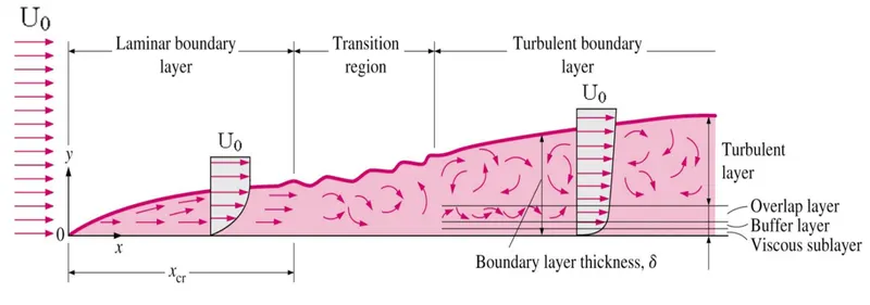
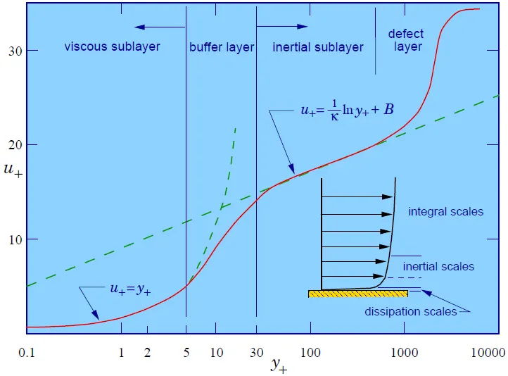
- First layer thickness calculation procedure using Y+.
- `text(Density of fluid (air)) = rho = 1.225 text( Kg/m^3)`
- `text(Dynamic Viscosity) = mu = 1.841*10^(-5) = text( Kg/ms at 300K)`
- `text(Pipe internal Diameter) = D = 0.015 text( m)`
- `text ( Inlet Velocity ) V text( in m/s)`
- `text ( Air Temperature) = 300 text( K)`
- `text(Reynolds number ) = R_e = (rho*V*D)/mu`
- `text ( Skin friction coefficient) = C_f`
- `text(Laminar )= C_f = 0.664/(sqrt(R_e))`
- `text(Turbulent )= C_f = 0.027/((R_e)^(1/7))`
- `text ( Wall shear stress) = tau_w = (C_f*rho*V^2)/2`
- `text ( Frictional velocity) = mu_f = sqrt((tau_w)/(rho))`
- `text (First Layer Thickness) = Y = (Y^+ *mu)/(mu_f*rho) text(m)`
First layer thickness calculation Procedure:
-
# Air properties rho = 1.225 # Density Kg/m3 mu = 1.846e-5 # Dynamic viscosity kg/m-s at 300K Re = 7000 # Renoulds number D = 0.015 # Diameter m y = 30 # Y+ # V = Inlet Velocity m/s #Re = (rho*V*D)/mu V = (Re*mu)/(rho*D) print(V) # Skin friction co-efficient C_f = 0.027/pow(Re,1/7) # Wall shear stress T_w = 0.5*C_f*rho*pow(V,2) # Frictional velocity U_f = (T_w/rho)**0.5 # first layer thickness Y = ((y*mu)/(U_f*rho)) # m print('First layer thickness = ', Y, 'meters') 
Geometry preparation in CONVERGE CFD:
-
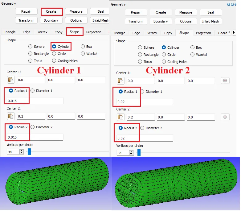
- Base Geometry:
- Creating 2 concentric cylinders
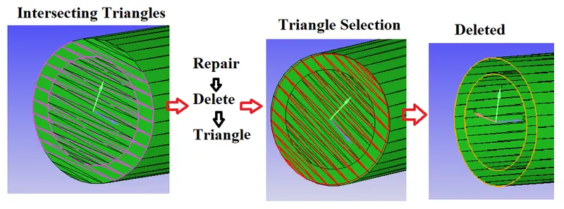
- Deleting intersecting triangles:
- Side face triangles of these cylinders are intersecting each other. We have delete the intersecting triangles.
- Go to Repair => Select the Intersecting triangles => Delete
- Repeat the same process for another side.
- Side face triangles of these cylinders are intersecting each other. We have delete the intersecting triangles.
- Creating additional triangles:
- To close open edges and to create an inlet and outlet we have to add additional triangles.
- Creating side Faces:
- Create => Triangle => Loft edges => Select First and Second set of edges => Apply
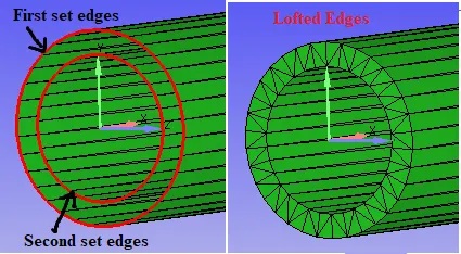
- Repeat the same process for another side
- Creating inlet and outlet faces:
- Repair => patch => list of edges => select edges => Apply
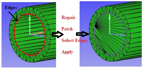
- Repeat the same process for another side
- Creating side Faces:
- To close open edges and to create an inlet and outlet we have to add additional triangles.
- Boundary setting:
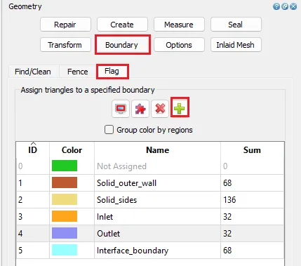
- Create boundary fences were ever required for proper section of triangles.
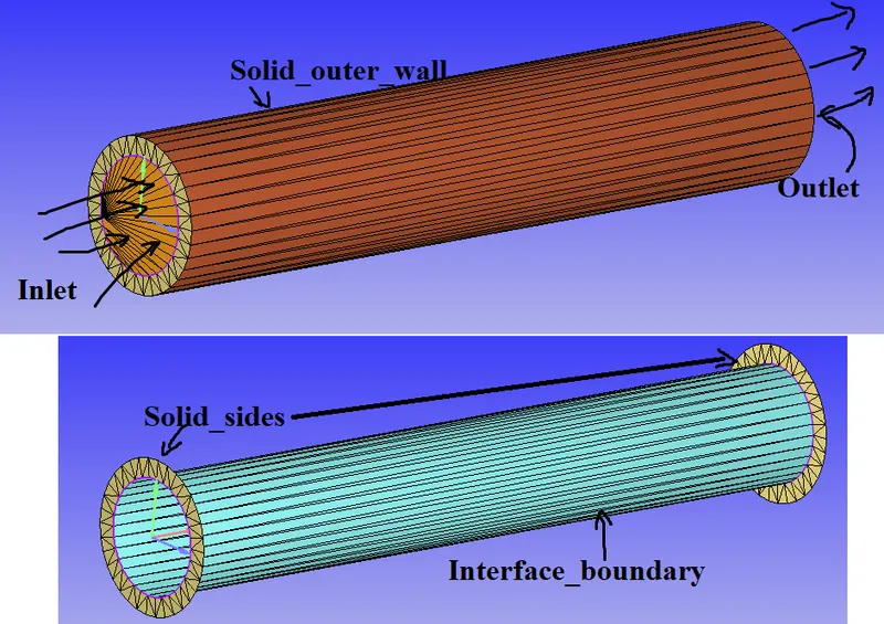
- By default In CONVERGE, all the surfaces are made up of triangles we have to select respective triangle faces for the boundary.
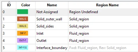
- Boundaries for the above-created geometry.: Inet, Outlet, Solid_outer_wall, Solid_sides, and interface boundary.
- Normal Transformation:
- All the face normal directions should be facing towards the flow region.
- In this fluid is flowing through the channel but normals are facing outwards. We have to transform the normal's direction.
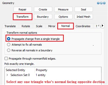
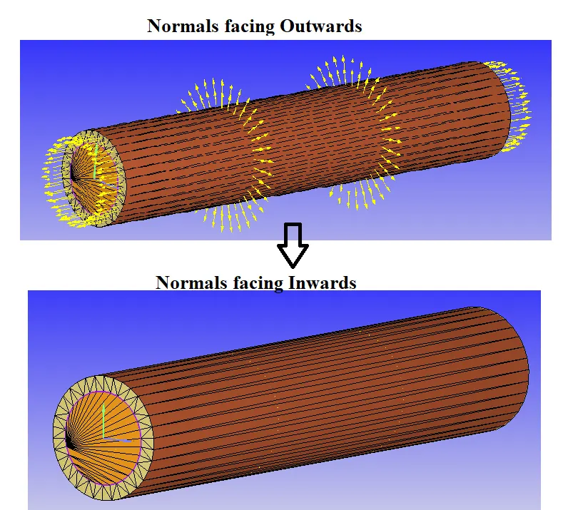
- Base Geometry:
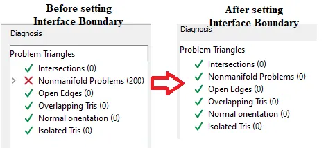
- Diagnosis:
- Checking for any interactions, open edges, Nonmanifold Problem etc.
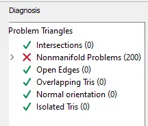
- This error is due to sharing of an edge by 3 different triangles.
- Boundary edges of the inlet face have been shared by Inlet, Solid_sides and Interface boundary.
- Dont care about this error it will go away while setting the case.
Case Setup in CONVERGE CFD:
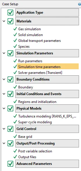
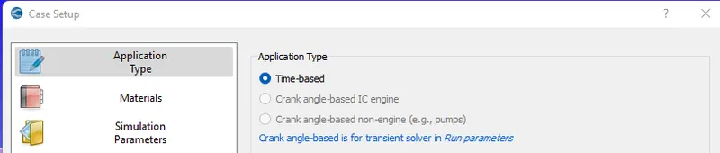
- Application Type :
- Materials:
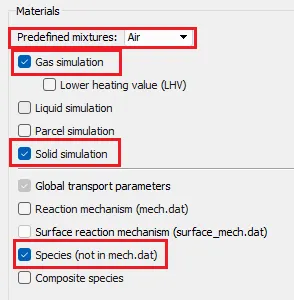
- Un check the reaction mechanism because in this problem there is no combustion reactions taking place.
- Defining Gas material:
- Gas: Add Gas species O2 & N2.
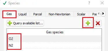
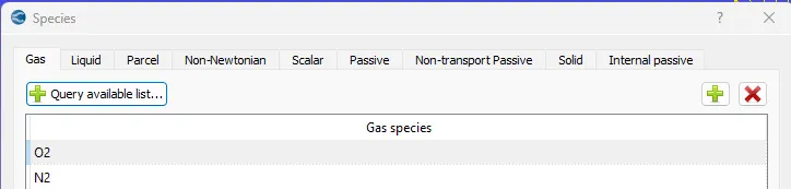
- Set default values in Gas Simulation & Global transport parameters.
- Defining Solid material:
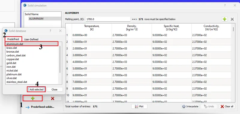
- Add Aluminum metal to Solid simulation

- Defining Gas material:
- Initial Conditions and Events:
- Regions and initialization:
- Adding Fluid and Solid region in regions section. initialize them them
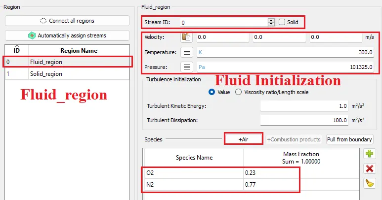
- Fluid_region:
- Steam Id = 0 ;
- Initialization :- Temperature = 300 K ; Pressure = 101325 Pa
- Add O2, N2 species.
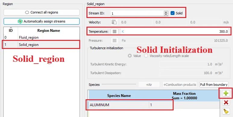
- Solid_region:
- Steam Id = 1 ; enable solid
- Initialization :- Temperature = 300 K.
- Add Aluminium material
- Regions and initialization:
- Boundary conditions:
- Defining boundary type and conditions:
-
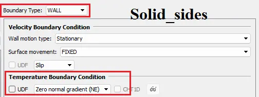
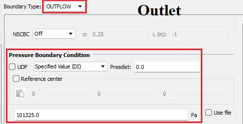
Boundary Name Type Boundary Condition Value Species Solid_outer_wall WALL Total Pressure Aluminium Solid_sides WALL Pressure Aluminium Inlet INFLOW Dirichlet B.C V_x = 7.03 Outlet OUTFLOW Dirichlet B.C Interface_boundary Interface - Solid_outer_wall:
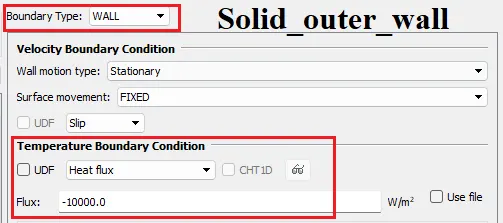
- Slip wall, Heat flux = -10000 W/m^2. -ve indicates heat flowing into the system.
- Solid_sides:
- Adiabatic Slip wall, heat transfer = 0. i.e, zero normal gradient.
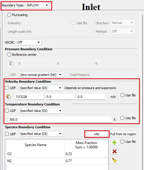
- Inlet: For inlet Dirichlet Boundary condition
-
`text(Density of fluid (air)) = rho = 1.225 text( Kg/m^3)`
-
`text(Dynamic Viscosity) = mu = 1.841*10^(-5) = text( Kg/ms at 300K)`
-
`text(Pipe internal Diameter) = D = 0.015 text( m)`
-
`text ( Inlet Velocity ) V text( in m/s)`
-
`text ( Air Temperature) = 300 text( K)`
-
`R_e = (rho*V*D)/mu = 7000`
- `(70000X1.841*10^(-5))/(1.225X0.015) = 7.03238 m/s`
-
- Outlet: For outlet Dirichlet Boundary condition atmospheric Pressure
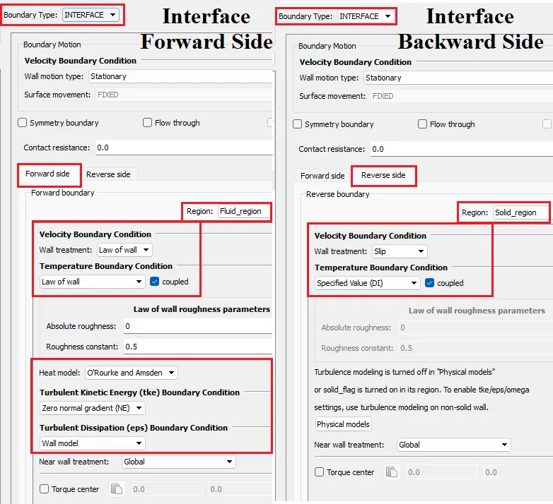
- Interface Boundary:
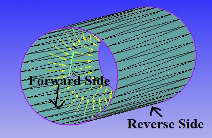
- This boundary is called the interface boundary because it was shared by two different regions.
- Forward Side: The boundary facing the direction of the normal vectors is called the Forward boundary.
- Reverse Side: The opposite direction of the normal vectors is the reverse boundary
- Solid_outer_wall:
- Note:
- After setting the interface boundary Nonmanifold Problem will gets resolved.
- Defining boundary type and conditions:
- Simulation Parameters:
- Run Parameters:
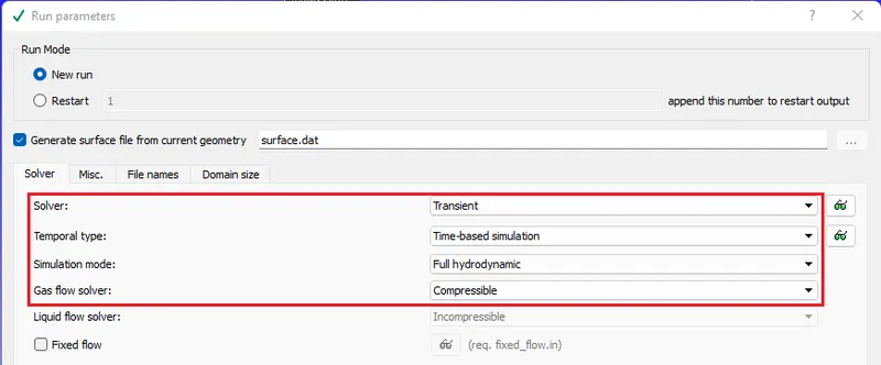
- Selecting the Solver & solver type. informing additional things to solve (Energy & Momentum equations).
- Although the Mach number is less than 0.3, We have to consider it as Incompressible and use a pressure-based solver. But, coverage is not that good enough to produce quality results when we use this combination.
- i.e, we are assuming it as compressible flow and using Density-based solver.
- Simulation Parameter:
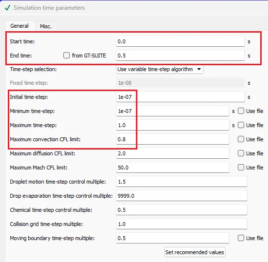
- defining star, end time, Minimum & Maximum Timestep sizes.
- Simulation Time calculation.
- From steady state analysis we got inlet velocity as 120 m/s
- length of the domain L is 0.2
- Time = Distance / Velocity
- T = 0.2 / 7.03238
- T = 0.0284
- So simulation time should be greater than 0.0284 sec
- For this analysis, we have taken simulation time as 0.5 seconds.
- Time = Distance / Velocity
- Solver Parameters:
- Solver Scheme to PISO and Density-based solver.
- under Equations window set precondition to None for all the variables.
- Navier-Stokes Solver Scheme: PISO
- Navier-Stokes solver type = Density-Based.
- Run Parameters:
- Grid Control:
- This is the section where we define meshing size(Grid size).
- Case 1 : dx = 0.004 m, dy = 0.004 m, dz = 0.004 m
- Case 2 : dx = 0.002 m, dy = 0.002 m, dz = 0.002 m
- Case 1 : dx = 0.004 m, dy = 0.004 m, dz = 0.004 m
- This is the section where we define meshing size(Grid size).
-
- Physical Models:
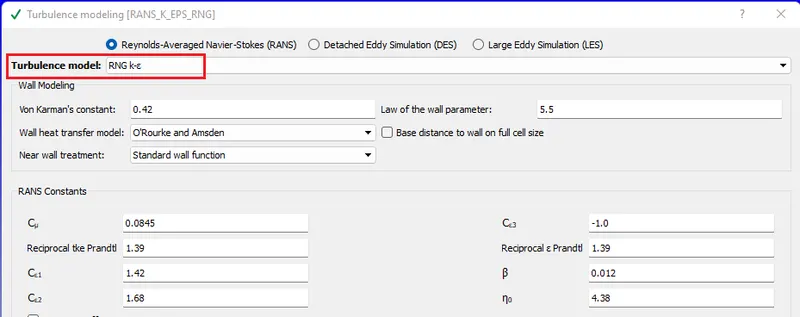
- Turbulence Modelling:
- using Renoulds Average Navier stroke equation
- The first cell away from the wall shall be placed at a y+ of 30-300.
- Turbulence Modelling:
- Super Cycle Modelling:
- Setting Steady-state solver for Solid.
- Begin storing super cycle data = 0.05 s. second Steady state solution recorded after 0.05 seconds.
- Time length for each cycle stage = 0.05 s. Steady state calculation done at every 0.05 seconds
- Conduction CFL number = 100
- SIE(Sensible internal energy) relaxation factor for super-cycle = 1.4
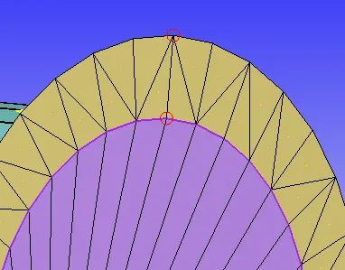
- We have to create a monitor point In solid body closer to Outlet.
- Measure => Diections => Two vertices => Selct Two vertices
-
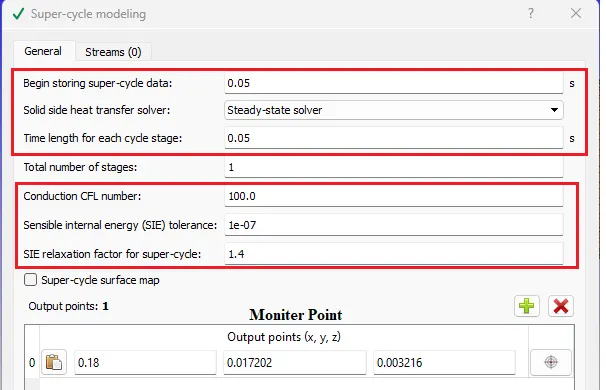
- Case 3 : Time length for each cycle stage = 0.03 seconds.
- Case 4 : Time length for each cycle stage = 0.02 seconds.
- Case 5 : Time length for each cycle stage = 0.01 seconds.
- Setting Steady-state solver for Solid.
- Physical Models:
- Output/Post-Processing
- Post Variable selection: select the variables to be monitored for post-processing.
-
S.No Typical variables Geometry/Location 1 Density Region ID 2 Pressure 3 Temperature 4 Velocity 5 Mesh Quality 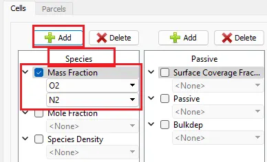
-
S.No Turbulence 1 Dissipation Rate of tke (eps) 2 Turbulent Kinetic Energy(tke) 3 Turbulent Viscosity 4 y+
-
- Post Variable selection: select the variables to be monitored for post-processing.


- Exporting Input files:
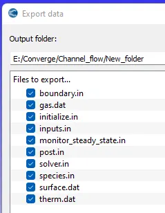
- Export the input files
- Export the input files
Solving Channel Flow in Cygwin:
- Go to the directory where input files are exported
- Make mpiexec.exe & converge.exe files globally available.
- "mpiexec.exe -n 4 converge.exe restricted </dev/null> logfile &"
- Use above mentioned line to start calculation in the background
- mpiexec.exe & converge.exe are executable applications to solve the problem
- -n 4:- number of processors
- restricted:- my license is a restricted one.
- </dev/null> logfile:- creates temporary memory to save data with name as logfile at a particular iteration
- & :- To run Calculation in Background
- "tail -10 logfile" command is used to view the last 10 lines of the logfile.
- "mpiexec.exe -n 1 post_convert_30_serial_64" command used to convert output files to paraview binary format, so that they can be processed in the paraview.
Post Processing and Results from Paraview:-
- open "..vtm" group file in paraview. This group contains all the solution files.
- use the slice tool to create a contour section plane and plot the contours
- Case 1 :
- dx = 0.004 m, dy = 0.004 m, dz = 0.004 m,
- Time length for each cycle stage = 0.05 seconds.
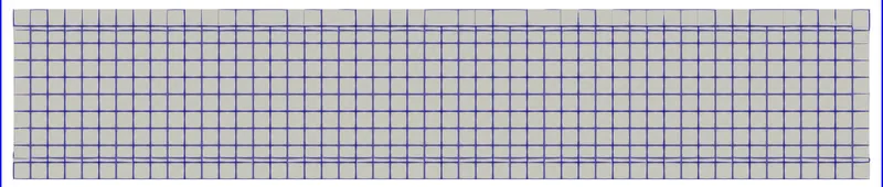
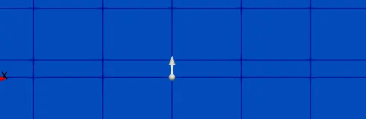
- Mesh:
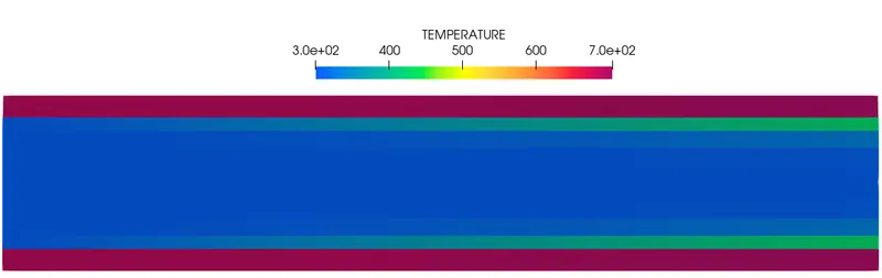
- Temperature Profile:
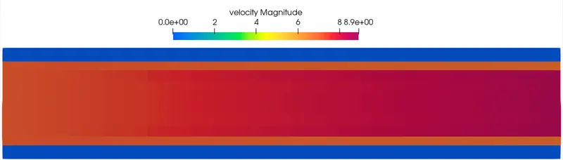
- Velocity Profile:
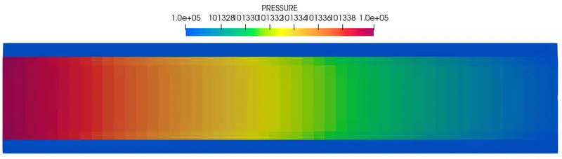
- Pressure Profile:
- Y+ = 0.001 m
- Case 2 :
- dx = 0.002 m, dy = 0.002 m, dz = 0.002 m,
- Time length for each cycle stage = 0.05 seconds.
- Mesh:
- Temperature Profile:
- Velocity Profile:
- Pressure Profile:
- Y+ = 0.000999 m
- Case 3,4,5 :
- dx = 0.002 m, dy = 0.002 m, dz = 0.002 m,
- Time length for each cycle stage = 0.03,0.02 & 0.01 seconds respectively.
- For all the cases contours looks similar.
- Temperature Profile:
- Velocity Profile:
- Pressure Profile:
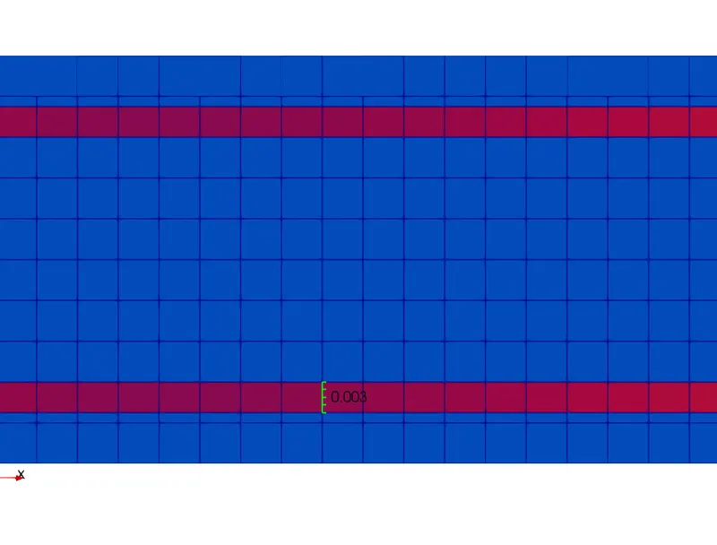
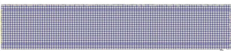
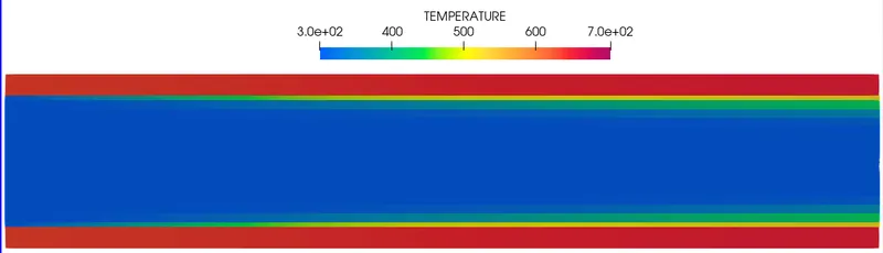
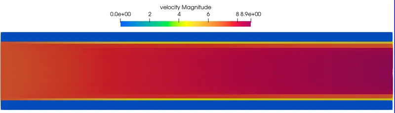
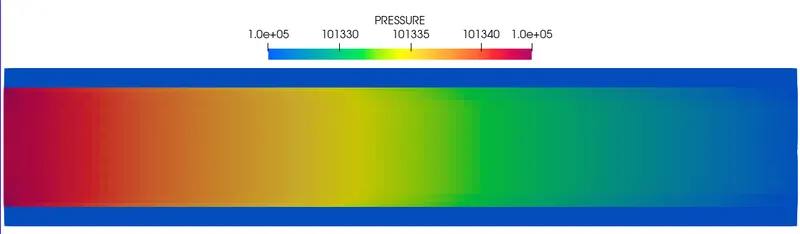

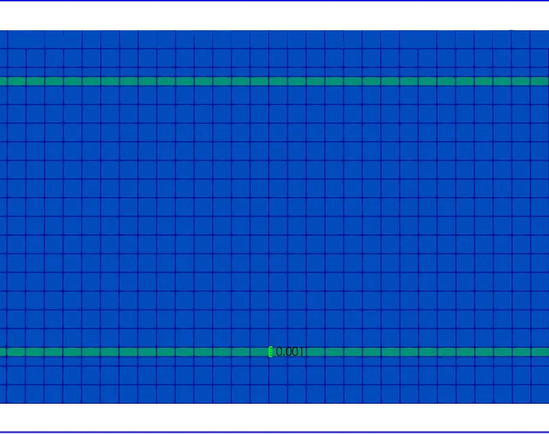
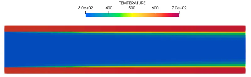
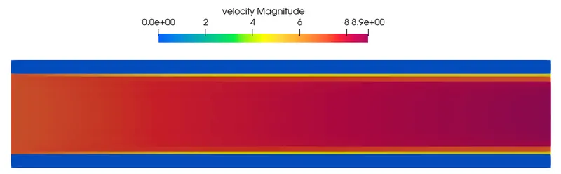
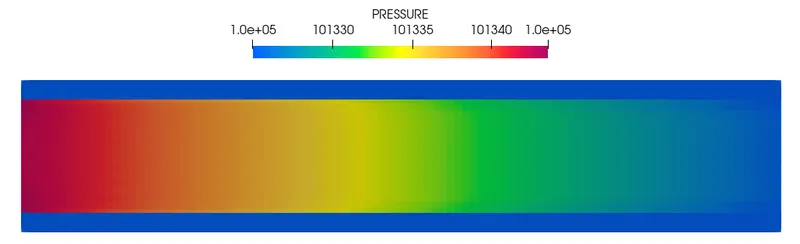
: Case 1,2
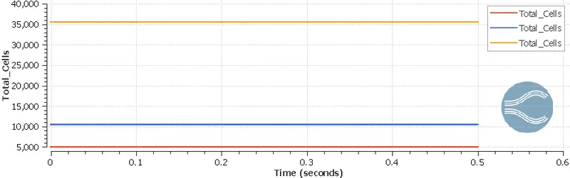
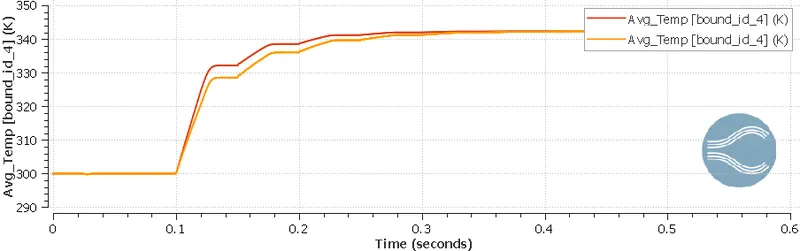
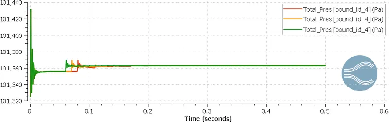
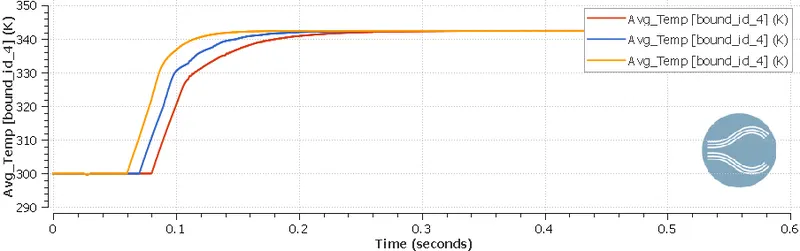
Plots to show the Effect of supercycle stage interval: Case 3,4 & 5.
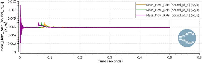
Conclusions:
- From Velocity contours, we can observe that Outlet velocity is greater than inlet velocity this is because air expanded due to the heating of pipe.
- As the mesh size decreases Y+ Value also decreases.
- From the Calculation, the First layer thickness should be less than 0.00104 meters for mech size 0.002 m satisfies the condition.
- From the Average Temperature plot of Case 3,4,5, we can observe that as the Time length of the Supercycle stage decreases Solution converges quickly.
How would you verify if the HTC predictions from the simulations are right
We use following emperical relation to validate Heat transfer co-efficient predictions from simulation they are:
Dittus-Boelter heat transfer coefficient correlation to calculate the nusselt number.
`text(Nusselt Number = )N_u = 0.023*R_(e)^0.8*P_r^n`
Validity:
- `0.6<=P_r<=160`
- `Re_(Dh)>10000`
- `L/D = 10`
- `text(Renoulds number = ) R_e = (rho*V*D)/mu`
- `text(Prandtl number = ) P_r = (mu*C_p)/k`
- We also that Nusselt Number `N_u = (h*l)/k`
- `h = (N_u*k)/l`
- `h = text(Heat transfer coefficient W/m^2-K)`
- `rho = text(Density kg/m^3)`
- `V = text(Velocity m/s)`
- `D = text(Diameter m)`
- `mu = text(Dynamic Viscosity kg/m-s)`
- `C_p = text(specific Heat of Fluid j/kg-K)`
- `k = text(Thermal conductivity of fluid W/m⋅K)`
- `text(For Cooling )n = 0.3`
- `text(For Heating )n = 0.4`
- `L = text(characteristic length D in m)`
Finally, `h text( )alpha text( ) N_u text( ) alpha text( ) R_e text( ) alpha text( )V`
Heat transfer coefficient is proportional to Nusselt number, Nusselt number is proportional to Renolds number which is directly proportional to flow Velocity.