Week 6: Conjugate Heat Transfer Simulation

Aim:

Setup a case in CONVERGE to perform Conjugate Heat Transfer simulation for a flow through a pipe.

• Perform a Grid dependence test on 3 grids and discuss outlet temperature converging value.
• With baseline configuration, study the effects of Supercycle stage intervals on total simulation time.
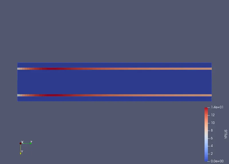
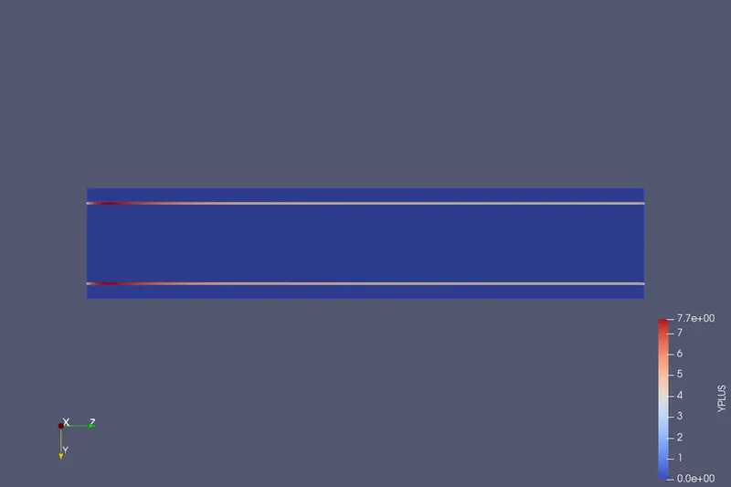
• Show contour plots for Y-plus, temperature, and velocity with Grid.

Introduction and Theory:

What is Conjugate Heat Transfer simulation?

The term conjugate heat transfer is used to describe processes that involve variations of temperature within solids and fluids, due to thermal interaction between the solids and fluids.

conjugate heat transfer (CHT) analysis can accurately predict heat transfer by simultaneously solving all the relevant solid and flow field heat transfer processes, for example, conduction through solids, free and forced convection in the gases/fluids, and thermal radiation.

The CHT approach has an advantage over FE thermal analyses in that wall heat transfer coefficients and their local variations on surfaces are directly calculated within the model rather than based on simplified empirical calculations. The CHT approach, therefore, has benefits for those applications where heat transfer is either non-uniform or difficult to calculate empirically.

In a simple world, you could simulate fluid flow and assume that the walls of the container were at a constant temperature or even adiabatic. In reality, however, the heat transfer between solids and surrounding fluids couples the temperature field in both materials, and thus your CFD software must be able to account for this phenomenon. CONVERGE features a state-of-the-art conjugate heat transfer (CHT) model for simultaneously predicting heat transfer in both the fluid and solid portions of the domain, which is critical for many applications.

Case Setup:

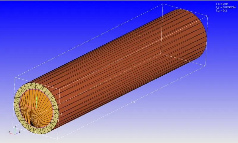
1. For this CHT use case, the following parameters are used to set up the case in CONVERGE Studio. This baseline configuration has

• Pipe Outer Diameter: 0.04 m.
• Pipe Inner Diameter: 0.03 m.
• Pipe Length: 0.2 m
  • 

2. Velocity boundary condition has to be calculated with given Inlet Reynold's number as 7000.

Re=(ρ⋅V⋅D)/μ

So, here,

Re = 7000

ρ = Density of air at 300K = 1.177 kg/m3

D = Diameter through which fluid is flowing = 0.03m

μ = Dynamic viscocity of air = 1.85e-5 kg/m-s

Thus,

V = Inlet Velocity = 3.6675 m/s.

This will be Dirichlet Inlet Boundary Condition.

3. This is a hollow pipe with outer solid material as Aluminium from a predefined library and the air is flowing through this hollow pipe with calculated boundary conditions.

4. The Boundary conditions are as follows:

Inlet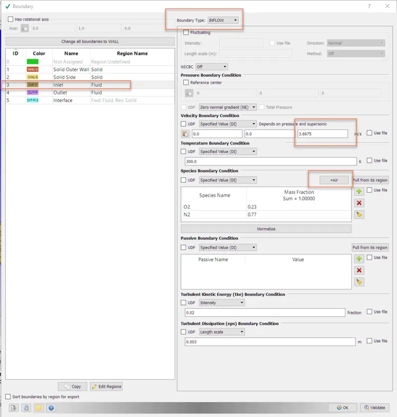
Outlet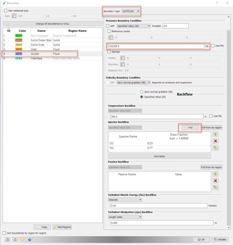
Solid Outer Wall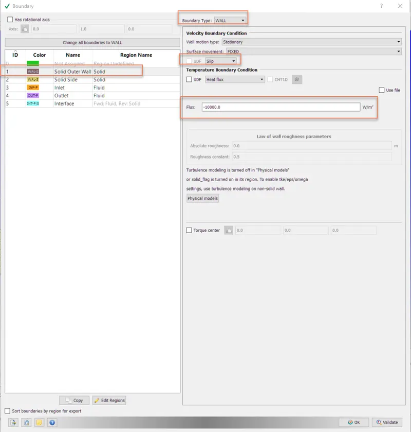
Solid Sidewall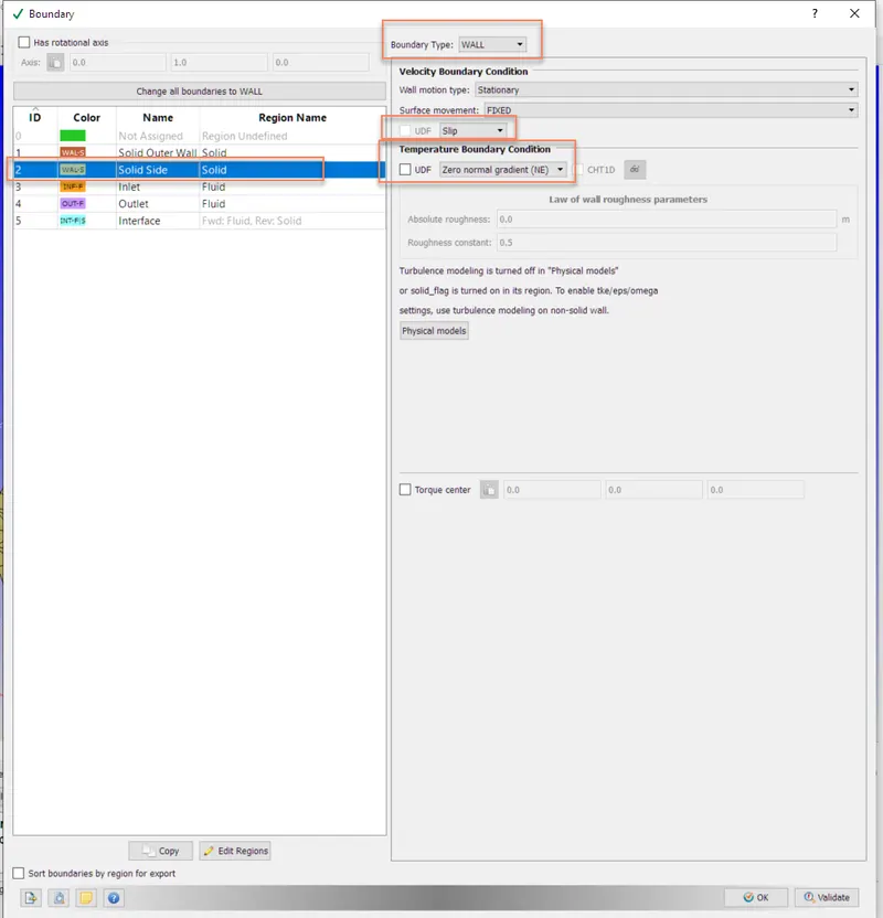
Interface Wall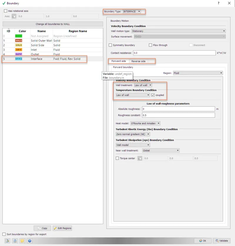

5. This particular simulation is running as a transient simulation from 0.0s to 0.5s with a minimum timestep as 1e-7.

6. We have created two regions. One for Solid and one for Fluid flow with different stream IDs.

7. For this setup, we are using RANS based K-ε turbulence model is used.

8. For conjugate heat transfer, in CONVERGE Studio we have to use a physics model named " Super-cycle modeling"

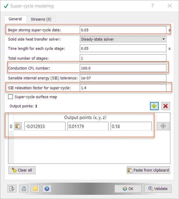
So what is super-cycle modeling?

There are several challenges when solving the fluid and solid domains together. The largest challenge to overcome is the difference in time scales associated with the heat transfer in the fluid and the solid. In general, heat transfer in the solid occurs more slowly than the convective and diffusive time scales of the fluid. This disparity in time scales is problematic for CFD simulations because simulations of long physical time periods can be computationally expensive.

CONVERGE offers an alternative approach called super-cycling for overcoming the time-scale disparity. In super-cycling, the fluid solver is frozen periodically while the heat transfer in the solid is allowed to progress to a steady-state. CONVERGE solves the fluid and solid phases in the same simulation without requiring you to stop and restart the simulation. Super-cycling significantly reduces the computational cost of the CHT simulation.

Another acceleration strategy in CONVERGE is the fixed flow method, which is useful for cases in which the flow changes less rapidly than other physical phenomena in your computational domain. By freezing the flow field and solving the flow for only short periods of time, the computational expense of the simulation is reduced. This is particularly beneficial for cases that require simulating a long period of physical time.

9. After setting up the grid size, variables for post-processing were selected. (velocity, mass flow, pressure, density, temperature)
10. After exporting input files, using CYGWIN (command prompt) was used to simulate the project setup.
11. Output files were later converted using CONVERGE studio for post-processing in ParaView.

Animation:

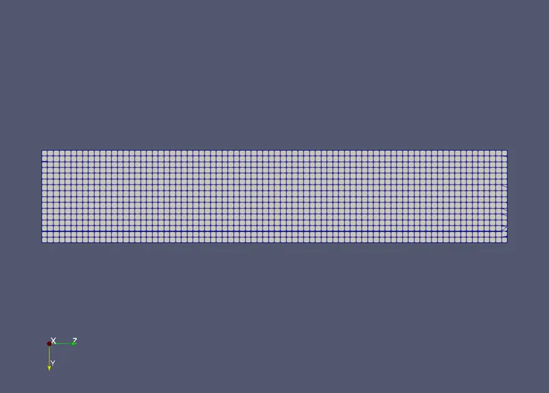
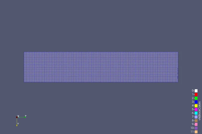
Objective 1: Perform a Grid dependence test on 3 grids and discuss outlet temperature converging value. (Grid dependence test)

Grid Size	0.004m	0.0025m	0.001m
Mesh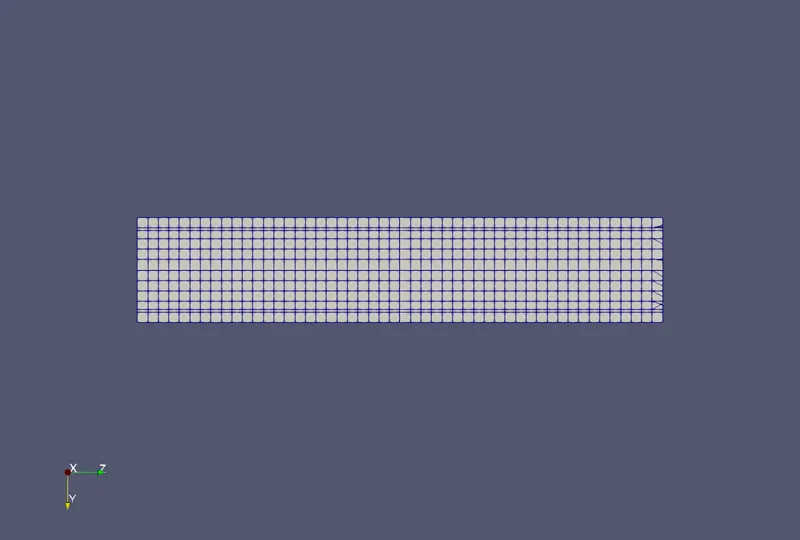
YPlus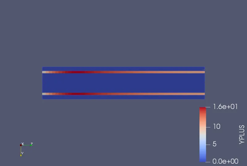
Temperature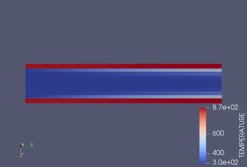
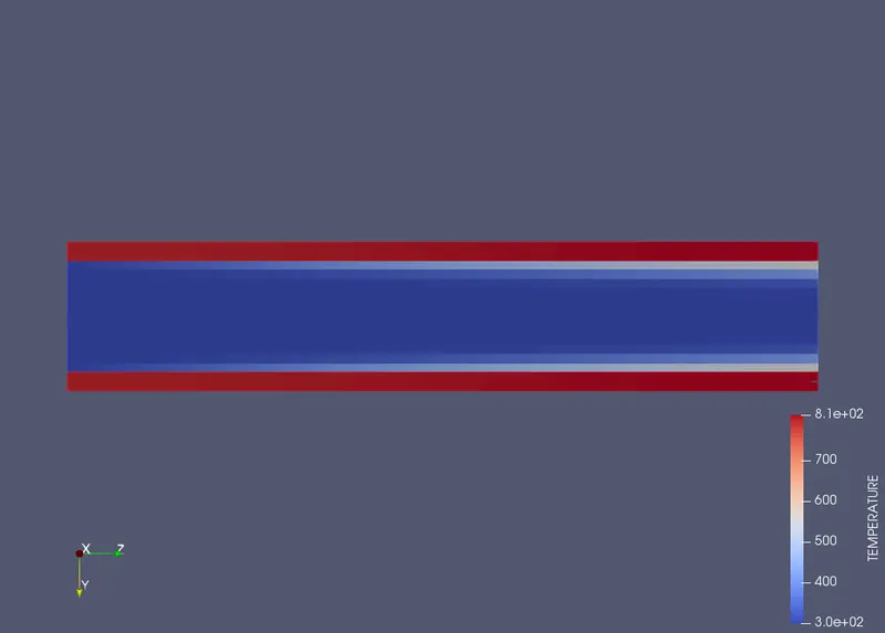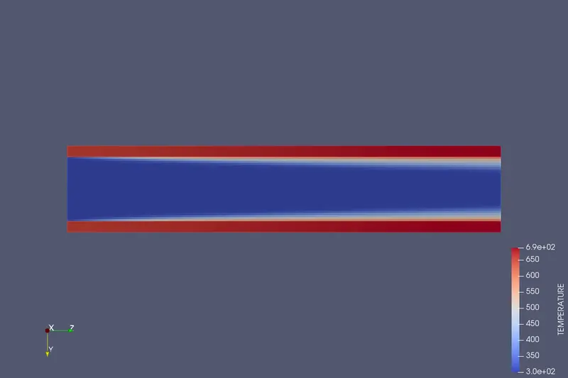Velocity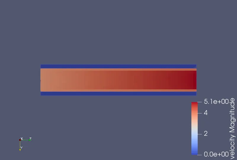
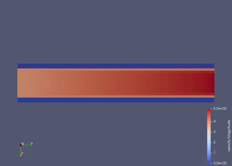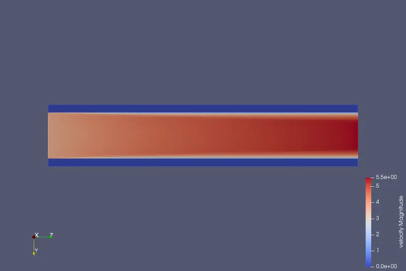Mean Temp (Solid Region)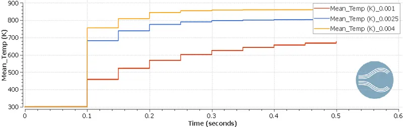
Temp Converging Value (Solid Region)	667.283K	803.328K	860.34K
Mean Temp (Fluid Region)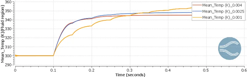
Temp Converging Value (Fluid Region)	345.02K	348.006K	353.819
Computation Time	199.798296 seconds	840.451790 seconds	37185.494820 seconds
Total Cell count	5000	17280	262400
No. of Cycles	2842	4443	14652

Objective 2:

With baseline configuration, study the effects of Supercycle stage intervals on total simulation time.

Super-cycling Stage	0.01	0.02	0.03
Computation Time	655.164510 seconds	706.089982 seconds	720.623427 seconds
Grid Size	0.0025m	0.0025m	0.0025m
Total Cell count	17280	17280	17280
No. of cycles	4740	4666	4592
Mean Temp (Solid Region)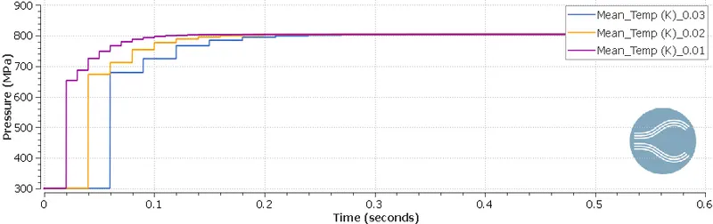
Mean Temp (Fluid Region)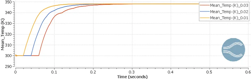

Summary of Results:

1. Yplus criteria is very important in Conjugate heat transfer analysis because it helps capture temperature and heat transfer coefficient.

2. As the base grid size is decreasing, the computation increases, the accuracy of results increases, the number of cycles for which simulation is running is increasing.

3. Also, with the increase in super-cycle stage parameters, computation time and the number of cycles decrease.

Conclusion:

A case has been set up in CONVERGE to perform Conjugate Heat Transfer simulation for a flow through a pipe.

• where we performed a Grid dependence test on 3 different grid sizes and discussed outlet temperature converging value.
• With baseline configuration, we studied the effects of Supercycle stage intervals on total simulation time.