CHT Analysis on a Graphics card
AIMS AND OBJECTIVES
- To perform a steady-state conjugate heat transfer analysis on a graphics card model.
- Run the simulation for three varying inlet flow velocities and compare the results.
- To find the maximum temperature and heat transfer coefficient observed at the processor.
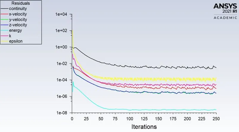
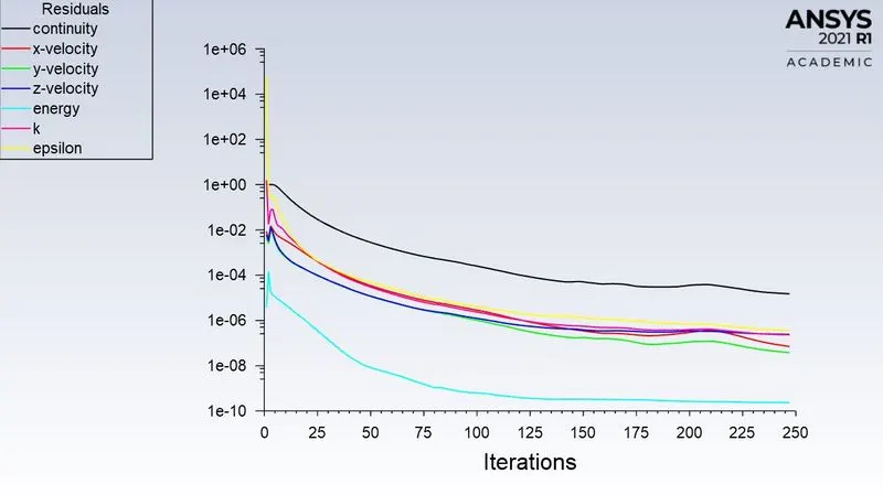
- To prove that the simulation has reached convergence with suitable plots and also, identity potential hotspots on the model.
Conjugate Heat Transfer:
The transfer of thermal energy from one region to another due to the temperature gradient is called heat transfer. When this heat transfer due to the exchange of thermal energy occurs across regions of multiphase, say, between solid and fluid, it is referred to as conjugate heat transfer.
Heat transfer in solid-phase occurs due to conduction and thermal conductivity describes the measure of heat conduction in solids. Whereas, heat transfer in fluid-phase is normally defined by convection. The level of convection is measured in terms of heat transfer coefficients.
Here, the steady-state simulation is performed on a graphics card. The graphic card is used in computers to help render images to the display hands down with faster math calculations and because of the same reason, the main GPU or processor heats up heavily. The fins used help transfer the heat generated in the processor by conduction and the same is transferred to atmospheric air by convection. The convection here is forced convection as we are using a certain velocity to the airflow.
The share topology of the graphics card is enabled to make sure the mesh is conformal.
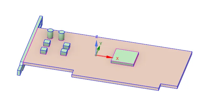
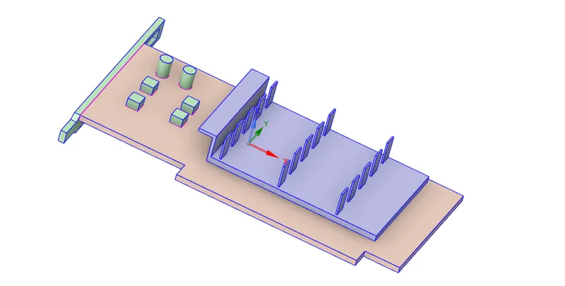
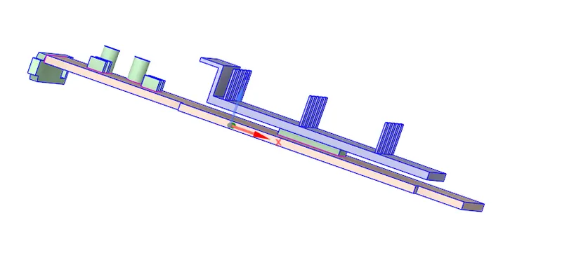
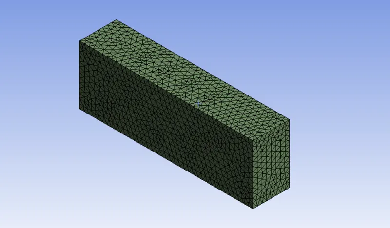
Meshing: The mesh sizes are a compilation of both coarse and refined at places in this geometry depending on their importance in physics. The heat transfer at the processor has to be captured well and hence the element size of the same has to be kept more refined. The fins are also in close contact with the processor for conduction as well as for convection and therefore the same has to be refined at optimum level. The mesh size at the remaining parts could be used as coarse as their involvement in the physics is not greatly taken into account. Below are the mesh sizes which are used in this simulation.
Element size of Enclosure = 5 mm
Element size of processor = 0.5 mm
Element size of fin and base = 1 mm
Element size of components on the base = 0.5 mm
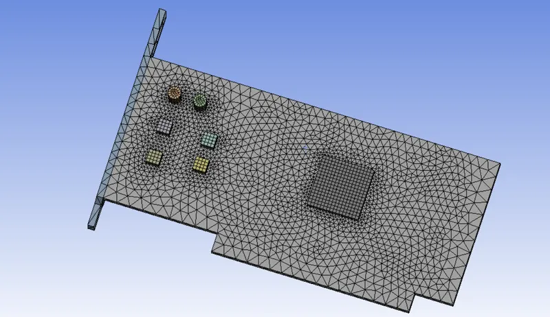
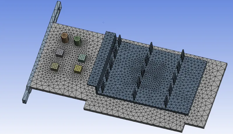
The materials used for different parts in the graphics card in this simulation are aluminium for the processor, copper fins and wood for the base. The processor is assumed to have a power density of 312500000 W/m³ by giving a source term there.
- Case 1: when inlet velocity is 5 m/s
Convergence Plot:
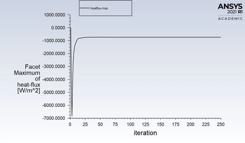
Heat Flux Plot:
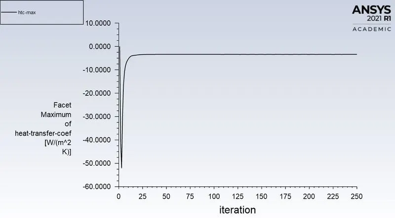
Surface Heat Transfer Coefficient Plot (Processor Wall):
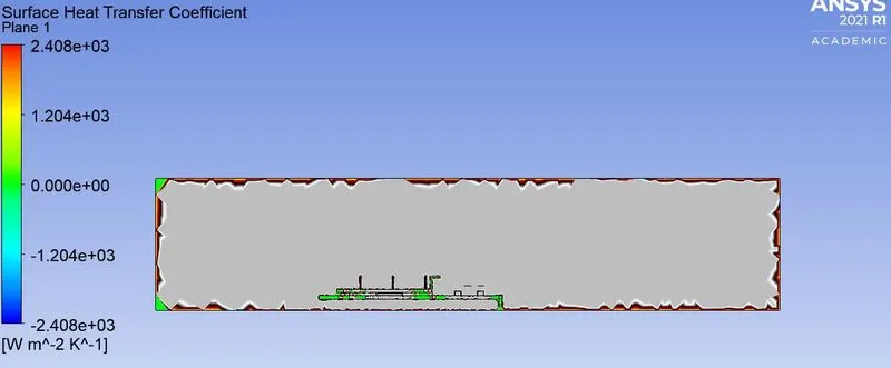
Surface Heat Transfer Coefficient Contour:
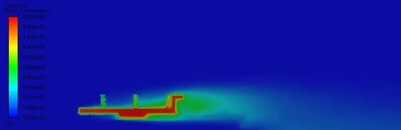
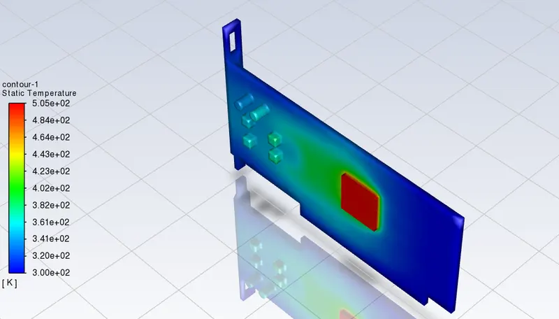
Temperature Contour:
Velocity Contour:
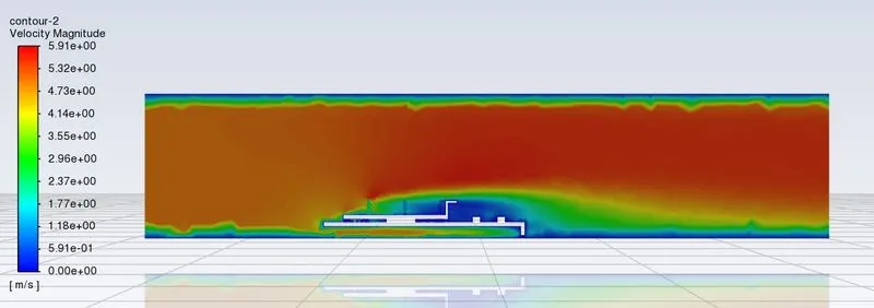
Maximum heat flux observed = -733.1709 W/m².
The maximum temperature at the processor = 504.24408 K
Maximum Surface Heat Transfer Coefficient = -3.3999937 W/(m² K)
- Case 2:when inlet velocity is 3 m/s
Convergence Plot:
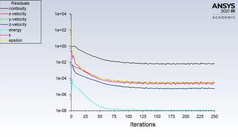
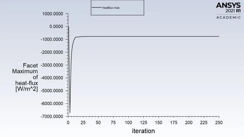
Heat Flux Plot:
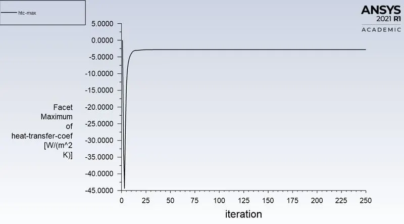
Surface Heat Transfer Coefficient Plot (Processor Wall):
Surface Heat Transfer Coefficient Contour:
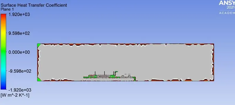
Temperature Contour:
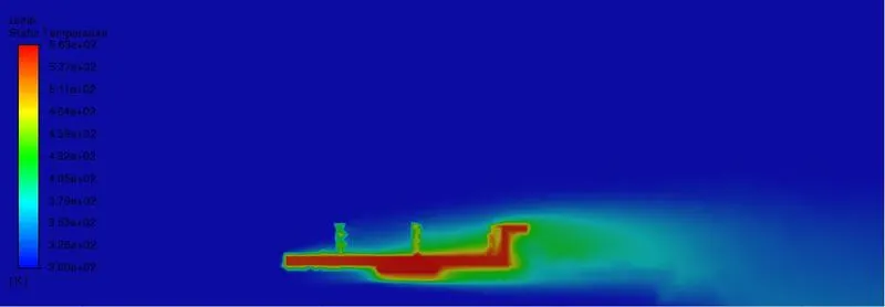
Velocity Contour:
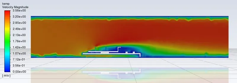
Maximum heat flux observed = -770.63593 W/m².
The maximum temperature at the processor = 562.83545 K
Maximum Surface Heat Transfer Coefficient = -2.8099055 W/(m² K)
- Case 3:when inlet velocity is 1 m/s
Convergence Plot:
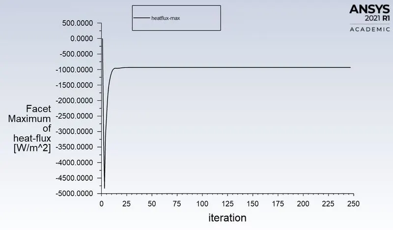
Heat Flux Plot:
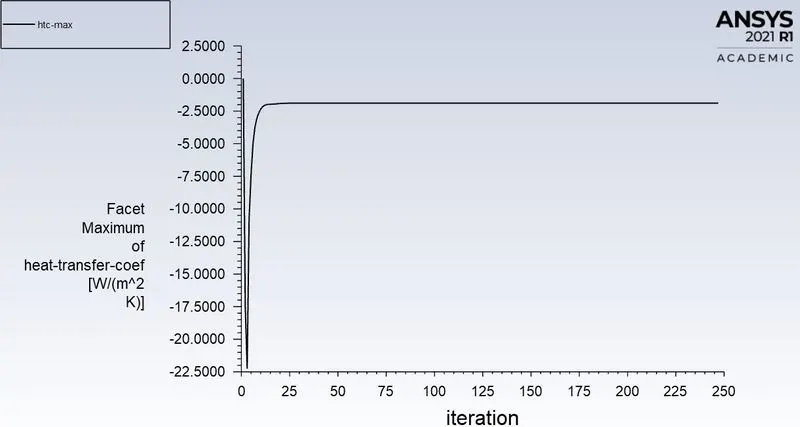
Surface Heat Transfer Coefficient Plot (Processor Wall):
Surface Heat Transfer Coefficient Contour:
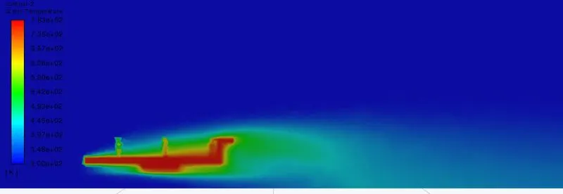
Temperature Contour:
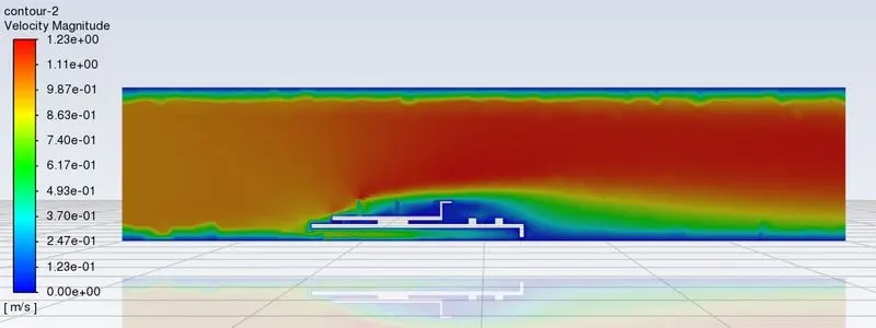
Velocity Contour:
Maximum heat flux observed = -932.09473 W/m².
The maximum temperature at the processor = 782.79938 K
Maximum Surface Heat Transfer Coefficient = -1.8859531 W/(m² K)
Inference:
- After the simulation is performed for different values of the velocity of air flow, that is, 1 m/s, 3 m/s and 5 m/s, it can be observed that the maximum temperature is 782.79938 K which is when the velocity is 1 m/s and similarly the maximum surface heat transfer coefficient is -3.3999937 W/(m² K) which is when the velocity is 5 m/s.
- Therefore, it can be learnt from the simulation that as the airflow velocity decreases, the corresponding value of the surface heat transfer coefficient decreases and the temperature exponentially increases.
- An increase in heat transfer coefficient means an increase in the conjugate heat transfer between the solids and fluids. Here surface HTC is maximum when velocity is 5 m/s and the respective temperature is also computed lower than the rest of the cases. Therefore, effective cooling can be provided at an increased velocity of airflow.