Week 6 - CHT Analysis on a Graphics card

CHT ANALYSIS ON A GRAPHICS CARD

AIM: Perform a steady-state conjugate heat transfer analysis on a model of a graphics card.

OBJECTIVE:

1. Simulate by varying the velocity from 1m/sec to 5m/sec for at least 3 velocities and discuss the results.
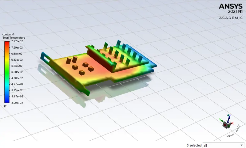
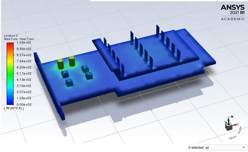
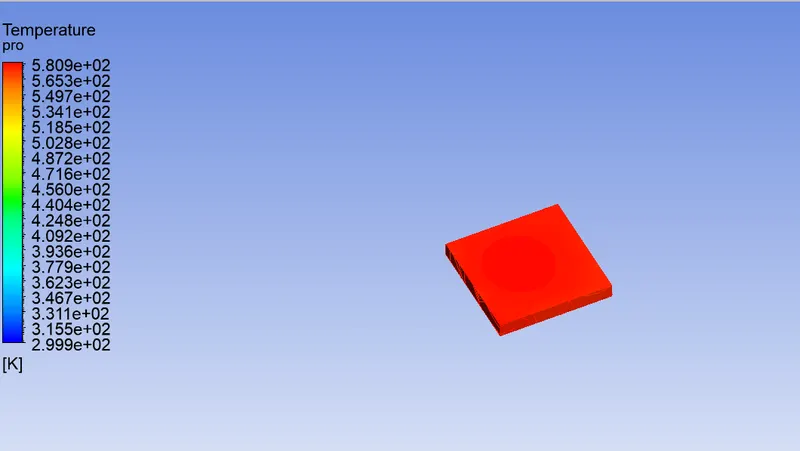
2. Find out the maximum temperature and heat transfer coefficient attained by the processor.
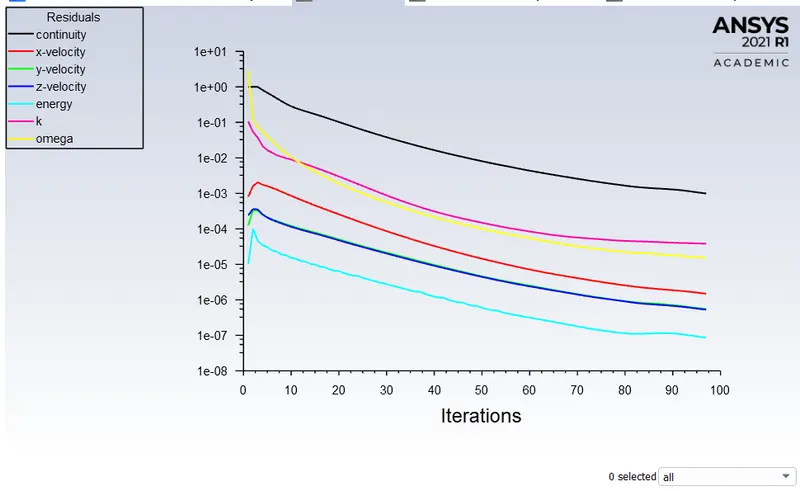
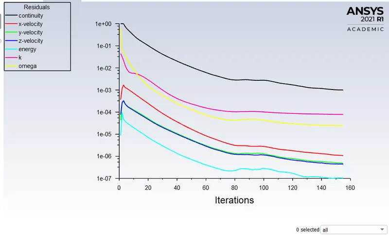
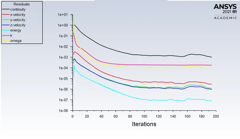
3. Prove that the simulation has achieved convergence with appropriate images and plots.
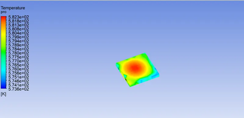
4. Identify potential hotspots on the model.

THEORY:

Conjugate Heat Transfer (CHT) Analysis:

Conjugate Heat Transfer analysis is used for the processes that involve a variety of temperatures concerning solids and fluids, due to thermal interaction between them. A typical example would be the heating or cooling of a solid by the flow of air.

The exchange of heat between two bodies is known as heat transfer and the rate of heat transfer is directly proportional to the temperature difference between them. Heat transfer in solids is usually occurred by conduction whereas in the case of fluids heat transfer occurs by convection. Efficiently combining heat transfers between solids and fluids is the key to design effective coolers, heaters, or heat exchangers. Forced convection is the most common way to achieve higher heat transfers. For some applications, the performance is further improved by combining convection with phase change(for example liquid water to vapor phase change).

Heat transfers in solid and heat transfers in fluids are usually combined in the majority of the applications. This is because fluid flows around solids or between solid walls and usually solids are immersed in the fluids.

An accurate description of parameters such as material properties, flow regimes, geometry configurations, selecting correct models based on the physics to be captured, heat transfer modes near the boundaries is needed for the analysis of temperature fields and heat transfer.

Practical CHT problems are used to determine:

• The maximum and minimum temperature in various parts of the system. eg: combustion chamber, gas turbines, chemical vessels, etc.
• Temperature Distribution is related to the thermal stress over a particular wall or system etc.
• Temperature Response in time-dependent applications such as heating/cooling problem (For example, In the case of cooling a particular system such as engine cooling)
• Overall heat transfer co-efficient.

SIMULATIONS AND PROCESS:

This project is divided into 2 parts based on the Mesh ( with a baseline and an upgraded mesh )

Again in Part 1, we run 3 different simulations with 3 different velocities 1m/s to 5m/s(using updraged mesh).

PART 1:

The geometries in both parts of the project are the same.

CASE 1:

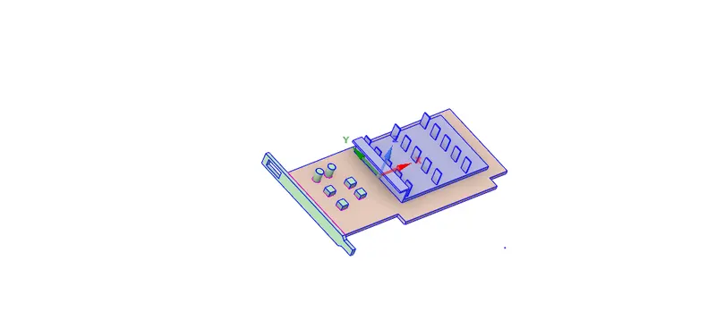
GEOMETRY:

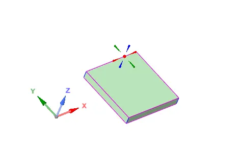
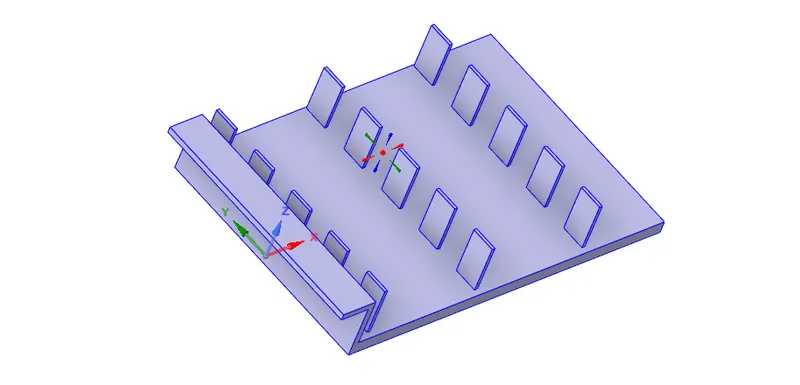
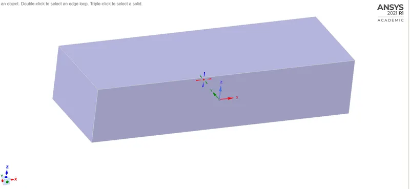
Using the given geometry, have to share the topology to reduce the interferences with:

1. Processor

2. Fins

3. Base

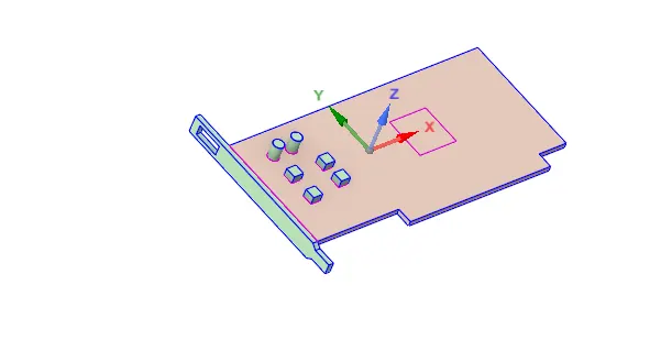
4. Encloser

5. Graphic card

MESH:

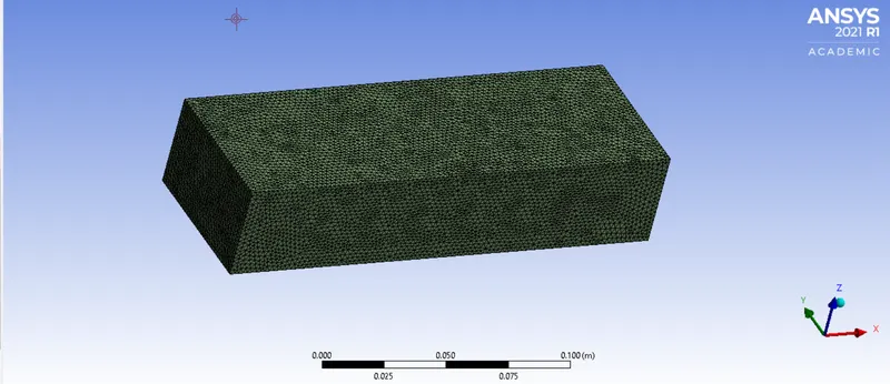
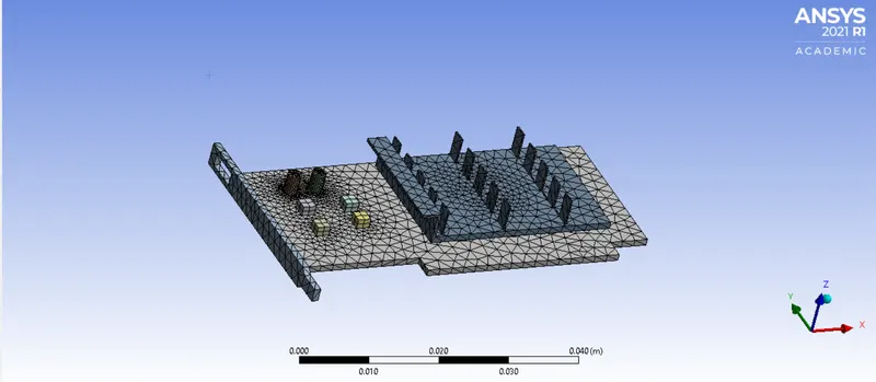
We start the mesh by naming the parts

1. Inlet

2. outlet

3. Wall symmetry

4. components

5. Fins

6. Base

7. Processor

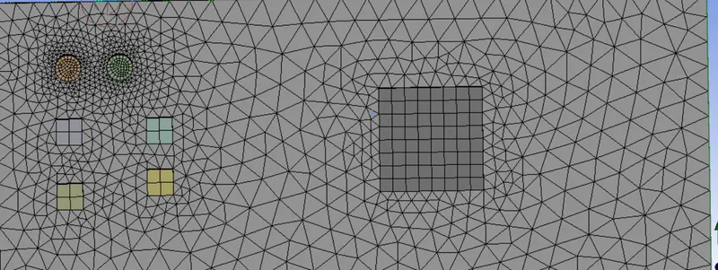
Then we give a total element size of 0.003 m and applying a body sizing to the processor with an element size of 0.0015. Making this our Refined mesh.

SIMULATIONS

SETUP
Solver Type	Pressure-Based
Velocity Formulation	Absolute
Time	Steady
Models	Viscous model: K-omega SST Energy model: On
Material	Fluid type: Air Solid-type: Aluminium : gold : copper
Cell zones	Fluid type: Air Solid: Al, Au, Cu
Boundaries	Inlet : inlet velocity: 2m/s : temperature = 300K Outlet: outlet pressure = 0
Reference values	Standard
Initialization	Standard

Usually, the power consumed by a processor is converted into heat energy. To calculate the heat generated on the processor which is = Power consumed divided by the total volume of the processor

"The power consumption of today's graphics cards has increased a lot. The top models demand between 110 and 270 watts from the power supply; in fact, a powerful graphics card under full load requires as much power as the rest of the components of a PC system combined"

Taking this fact we will assume the power consumed to be 55 (being half of the upgraded graphic card)

Heat generated = `55/(64*10^-9) W/m^3 = 859375000 W/m^3`

RESULTS:

Residual plots

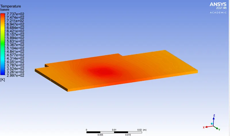
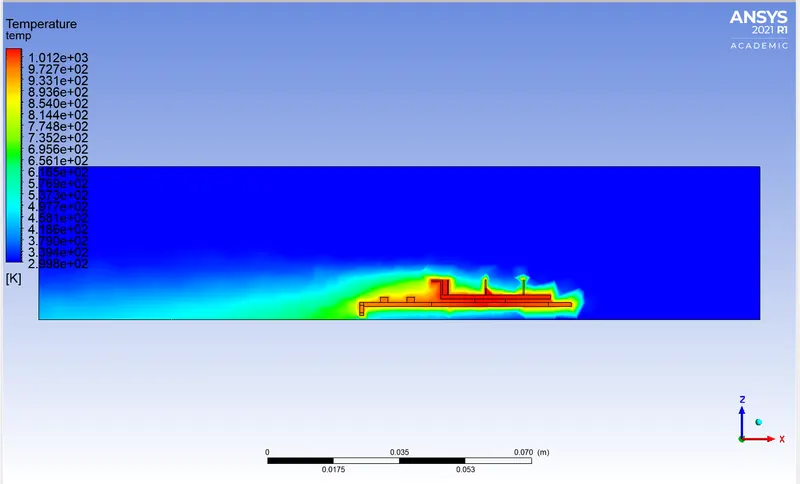
The temperature on the Graphic card

Wall heat transfer coefficient

Post Processing:

Temperature contour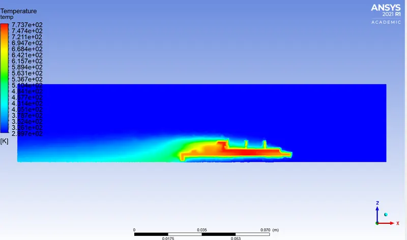

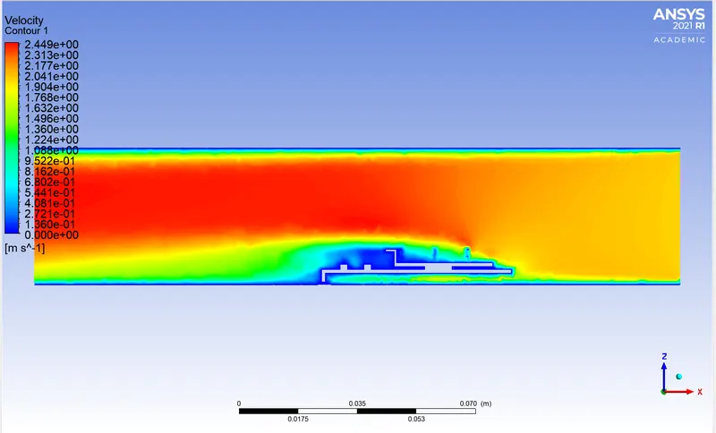
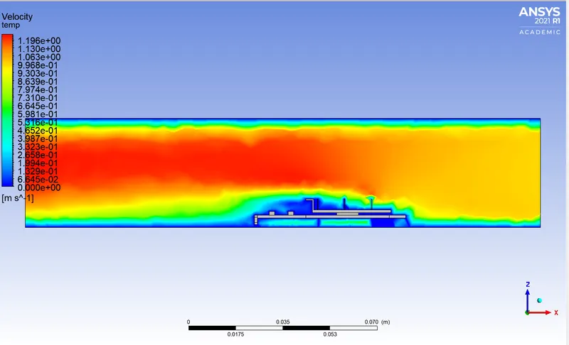
Velocity contour

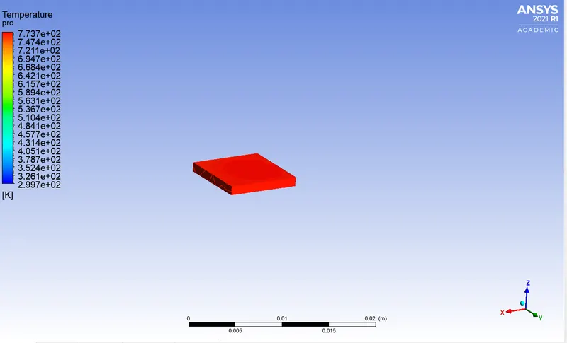
Temperature on processor

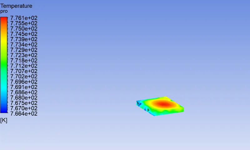
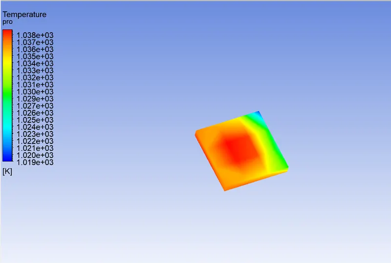
the temperature on the processor (local)

Temperature of fins

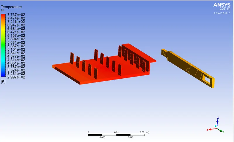
Temperature of Base

CASE 2:

SIMULATIONS

SETUP
Solver Type	Pressure-Based
Velocity Formulation	Absolute
Time	Steady
Models	Viscous model: K-omega SST Energy model: On
Material	Fluid type: Air Solid-type: Aluminium : gold : copper
Cell zones	Fluid type: Air Solid: Al, Au, Cu
Boundaries	Inlet : inlet velocity: 5m/s : temperature = 300K Outlet: outlet pressure = 0
Reference values	Standard
Initialization	Hybrid

RESULTS:

Residual plots

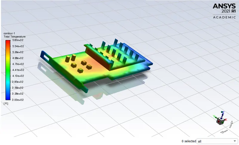
The temperature on the Graphic card

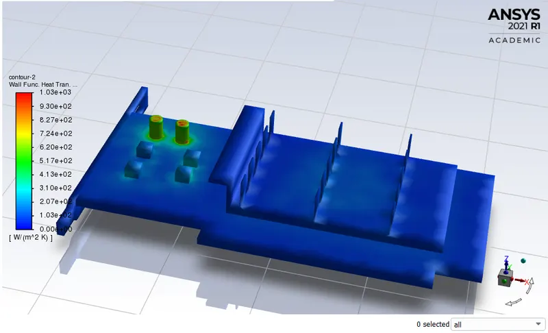
Wall heat transfer coefficient

Post Processing:

Temperature contour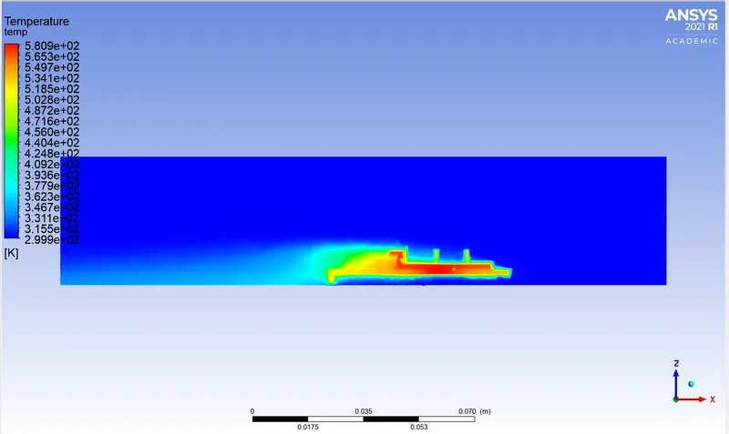

Velocity contour

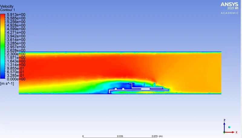
Temperature on processor

the temperature on the processor (local)

Temperature of fins

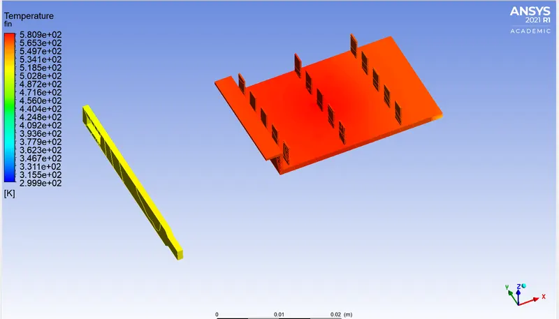
Temperature of Base

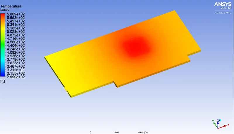
Show in case 3 and part 2 differences below :

PART 2:

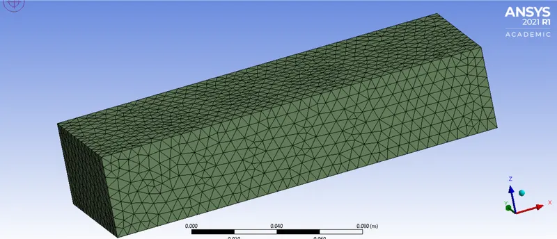
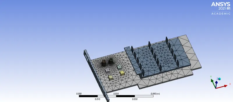
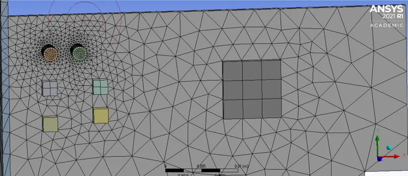
First, we'll show the mesh of part 2 which is our baseline mesh

MESH

Then we give a total element size of 0.005 m and applying a body sizing to the processor with an element size of 0.0025

and applying sizing for the components with curvature on. Making this our base mesh.

CASE 3 And PART 2:

SIMULATIONS

SETUP
Solver Type	Pressure-Based
Velocity Formulation	Absolute
Time	Steady
Models	Viscous model: K-omega SST Energy model: On
Material	Fluid type: Air Solid-type: Aluminium : gold : copper
Cell zones	Fluid type: Air Solid: Al, Au, Cu
Boundaries	Inlet : inlet velocity: 5m/s : temperature = 300K Outlet: outlet pressure = 0
Reference values	Standard
Initialization	Hybrid

RESULTS:

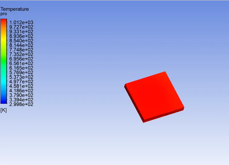
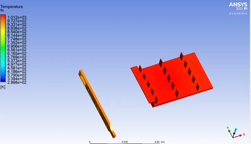
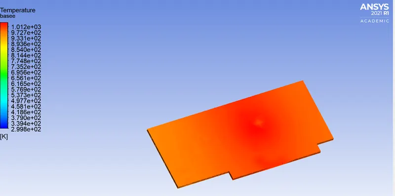
DIFFERENCE (with inlet velocity = 1m/s)	CASE 3(REFINED MESH)	PART 2(BASELINE MESH)
Residual plots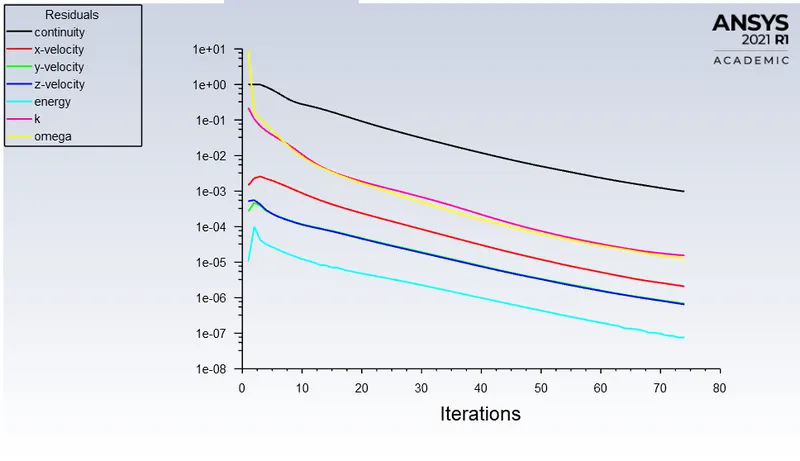
The temperature on the Graphic card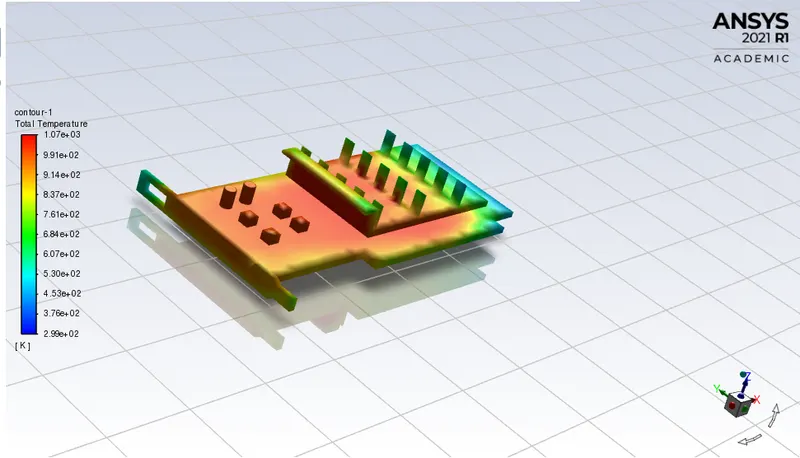
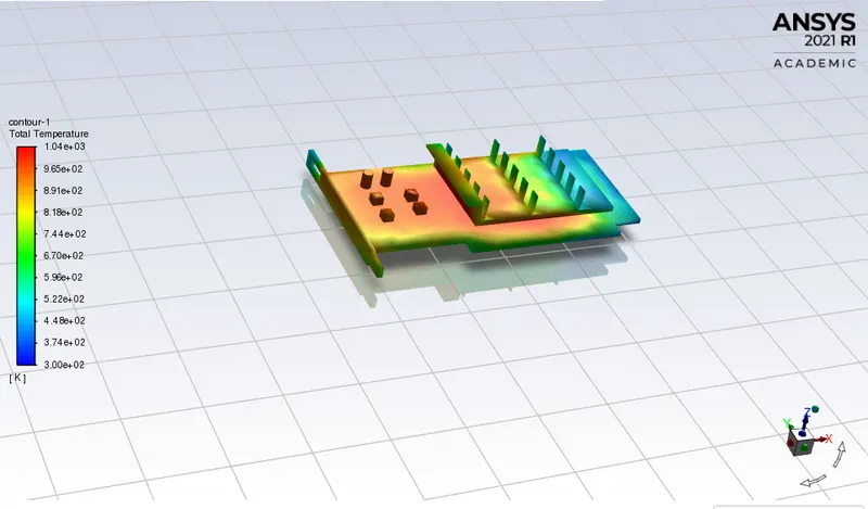Wall heat transfer coefficient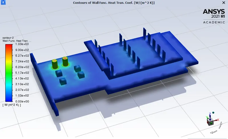
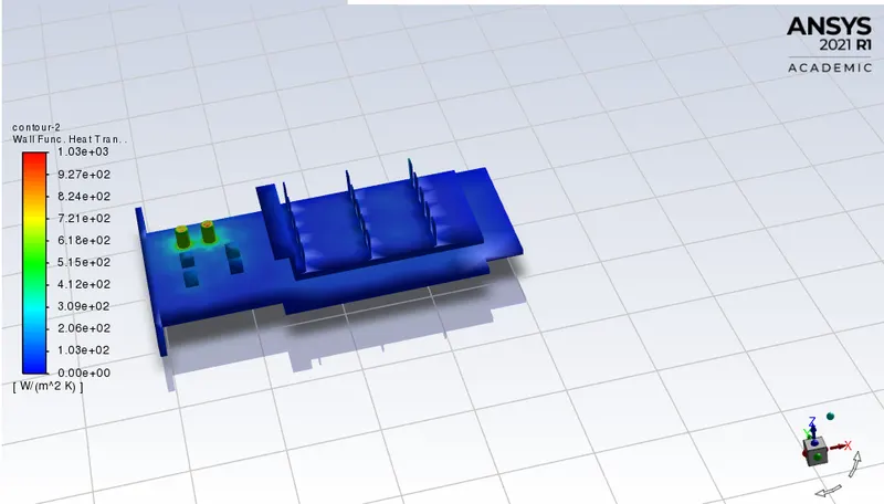Post Processing:
Temperature contour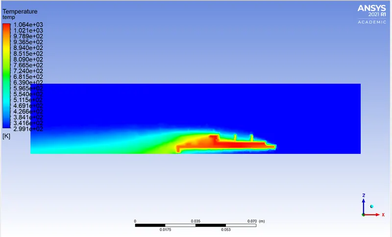
Velocity contour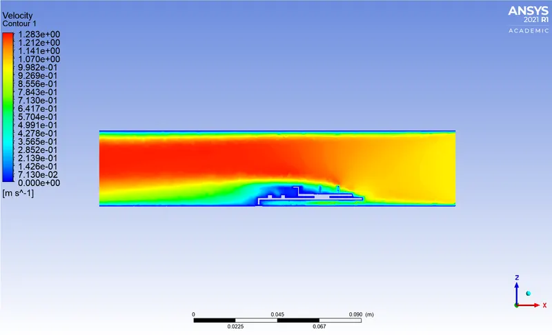
Temperature on processor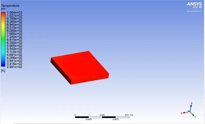
the temperature on the processor (local)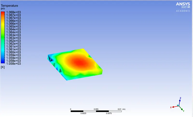
Temperature of fins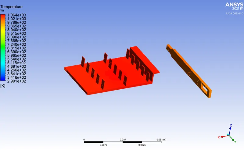
Temperature of Base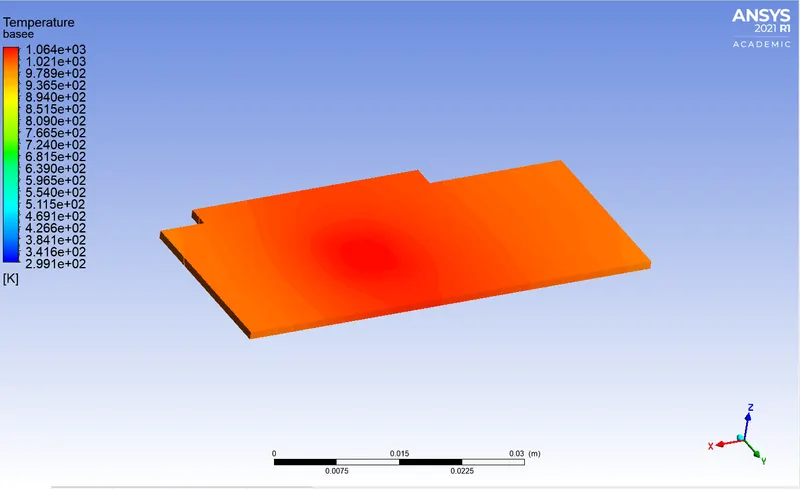

CONCLUSION:

CASES	VELOCITY(m/s)	TOTAL TEMPERATURE OF GRAPHICS CARD(K)	TOTAL HEAT TRANSFER COEFF ON GRAPHICS CARD (W/m^2K)
CASE 1	2	773	1030
CASE 2	5	583	1030
CASE 3	1	1070	1030
BASELINE MESH (part 2)	1	1040	1030

• Higher velocity in a particular region means a higher Reynolds number. That’s why the heat transfer coefficient in that area is highest, which means the maximum amount of heat transfer is taking place from fluid to the solid in that region. This also results in a higher temperature of solid in that location.
• Heat transfer coefficient is a function of properties of the fluid at film temperature, temperature difference, temperature coefficient, buoyance force et, hence, mesh resolution near walls usually has the biggest impact on numerical results.
• For the turbulent models, we have to take care of the assumptions and the boundary conditions you put in the program. The mesh is a very important parameter to get nice results so we have to refine it in the important place of our drawing.
• Some factors that should be considered which the most significant is the turbulent boundary layer. If we are using any kind of low Reynolds turbulence model considering enhanced wall treatment (as your K-w SST model), so we need to make sure that we stay in the laminar sub-layer region where velocity profiles are assumed to be laminar and viscous stress dominates the wall shear which means
• Mesh/ grid dependency test is very important to get confidence over results.