RESUBMITTING FROM LIVE CLASS CHALLENGE

CHT ANALYSIS ON GRAPHICS CARD

Aim :

• Perform a steady-state conjugate heat transfer analysis on a model of a graphics card. You can use appropriate materials of your choice for the simulation. Make sure to properly define the correct solid and fluid zones. Refer the video for further clarification and the model is provided below the video.
• Run the simulation for best possible mesh with combination of coarse and refined mesh in different regions. Explain the reason for choosing the particular mesh settings.

Objectives :

1. Run the simulation by varying the velocity from 1m/sec to 5m/sec for at least 3 velocities and discuss the results.
2. Find out the maximum temperature and heat transfer coefficient attained by the processor.
3. Prove that the simulation has achieved convergence with appropriate images and plots.
4. Identify potential hotspots on the model.

Theory :

1. Introduction:

• The main difference between thermodynamic analysis and heat transfer analysis is that in thermodynamic , we deal with system in equilibrium i.e. to bring a system from one eqb. State to another equilibrium state how much heat required is the main criteria. While in heat transfer analysis, we evaluate at what rate this change of system occurs by calculating rate of heat transfer in (J/s or Watt).
• Heat transfer is known as the flow of thermal energy from one region to another region occupied by any matter (solids and fluids) where the rate of heat transfer is proportional to the temperature difference between the regions/matters.
• Conjugate heat transfer (CHT) is used to describe the variation of temperature between the solids and fluids due to the exchange of thermal energy between them.

2. Modes of heat transfer :

• There are 3 ways of modes of heat transfer

1. Conduction
2. Convection
3. Radiation

2.1. Conduction :

• Conduction is the mode of heat transfer which generally occurs in solids due to temp difference associated with molecular lattice vibration energy transfer and also by free electron transfer.
• The reason behind all electrically good conductors are also in general good conductors of heat is that the presence of abundant (i.e. plenty) number of electrons available in the outermost orbit of atoms.

Ex : All metals.

• Notable exception to the above statement is Diamond (K=2300 W/m-K). The highest conductivity of diamond is due to perfect crystalline molecular lattice structure.

2.1.1. Fourier’s law of conduction :

• It states that,” the rate of heat transfer by conduction along a given direction is directly proportional to the temp gradient along that direction and is also directly proportional to the area of heat transfer lying perpendicular to the direction of heat transfer.”

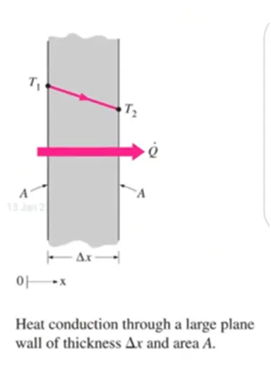
i.e. qx∝dTdx">` q x ∝ d T d x `Pr=MomentumD⇔usivityThermalD⇔usivity

And qx∝A">` q x ∝ A `Pr=velocityboundarylayerthick≠ssThermalboundarylayerthick≠ss

Now by combining these equations we can write as

qx=-KAdTdx">` q x = - K A d T d x `Pr=να=μρKρCp=μCpK

Where,

K= Thermal conductivity (W/m-K)

A = Normal surface area (m²)

dTdx">` d T d x `Re=I≠rtiaforce(Fi)viscousforce(Fv)= Temp gradient

q_x = Conductive heat transfer (Watt)

• Here the negative sign denotes heat transfer in the direction of decreasing temperature.
• Thermal conductivity is the measurement of materials ability to conduct heat.

2.2. Convection :

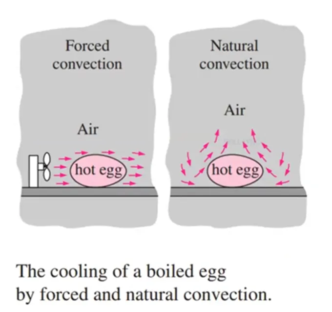
• Convection is the mode of heat transfer which generally occurs between a solid surface and the surrounding fluid due to temp difference associated with macroscopic bulk motion of the fluid transporting thermal energy in the form of enthalpy.
• In case of forced convection heat transfer this motion of fluid is provided by an external agency like a fan or blower or a pump where as in free convection heat transfer the motion of the fluid occurs naturally due to buoyancy forces arising out of density changes of fluid because of its temperature.

2.2.1. Newton’s law of cooling :

• The law states that, “the rate of heat transfer by convection between solid body and surrounding fluid is directly proportional to the temp difference between them and also directly proportional to the area of contact or area of exposure between them.”

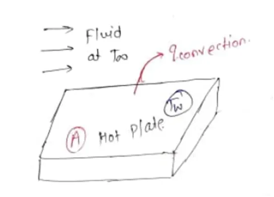
i.e. qconv∝(Tw-T∞)">` q c o n v ∝ ( T w - T ∞ ) `Re=ρVDμ=VDν

And qconv∝A">` q c o n v ∝ A `Eb∝T4

Therefore, qconv=hA(Tw-T∞)">` q c o n v = h A ( T w - T ∞ ) `Eb=σT4

Where,

h= convective heat transfer coe. (W/m²-K)

A= surface area of a solid body where fluid comes in contact (m²)

T_w = plate temp (K)

T∞">` T ∞ `= fluid or ambient temp (K)

• The convective heat transfer coe.(h) is not a property of the fluid. It is experimentally determined parameter whose value depends on all the variables influencing convection such as the surface geometry, the nature of the fluid motion, the properties of the fluid and the bulk fluid velocity.
• Typical values of h are given in table

Sr. no	Type of convection	h(W/m2-K)
1	Free convection in gases and vapours	3-25
2	Forced convection in gases	25-400
3	Free convection in liquids	250-600
4	Forced convection in liquids	600-4000
5	Condensation in heat transfer	3000-25000
6	Boiling heat transfer	5000-50000

2.2.2. Nusselt number:

• It is the ratio of convective heat transfer to conductive heat transfer within a fluid region.

Nu=Convective heat transferConductive heat transfer=hKL=hLk">` N u = Convective heat transfer Conductive heat transfer = h K L = h L k `

Where,

h = convective heat transfer coe. (W/m²-k)

K = thermal conductivity of a fluid (W/m-k)

L= thickness of a plate (m)

• Nusselt number denotes the increase in heat transfer through a fluid layer caused by convection, relative to conduction.
• When a fluid is motionless (i.e. no bulk motion), conduction will be the dominating mode of heat transfer (Nu=1).
• When a fluid is in bulk motion, the convection will be higher.

2.2.3. Prandtl’s number:

• It is the ratio of momentum diffusivity to thermal diffusivity.
• It compares the velocity boundary layer thickness to the thermal boundary layer thickness (which boundary layer is thicker).

Where

ν = Kinematic/momentum diffusivity (m²/s)

α = Thermal diffusivity (m²/s)

µ = dynamic viscosity (Pa-s)

C_p = sp. Heat (J/kg-K)

• Prandtl number is a dimensionless number.
• Prandtl number for gases is about 1, for water it is in the order of 10.
• It is 0.01 for liquid metals and 10⁵ for heavy oils.
• For air, Pr=0.65 - 0.71
• Local conv. Heat transfer coe. for laminar boundary layer over a flat plate can be determined from following empirical equation as,

Nu=hLK=0.664Re0.5Pr0.33">` N u = h L K = 0.664 R e 0.5 P r 0.33 `

• For fully developed turbulent flow through pipes or ducts , the heat transfer coe. Can be calculated as,

Nu=hDk=0.023Re0.8Prn">` N u = h D k = 0.023 R e 0.8 P r n `

Where,

n= 0.4, for heating of the fluid

n= 0.3, for cooling of fluid.

2.2.4. Reynolds number :

• The Reynolds number is a dimensionless number, named after the Osborne Reynolds , defined as the ratio of inertia forces to the viscous forces. Mathematically it is given as,

Inertia force(Fi)viscous force (Fv)">

i.e. Re=ρVDμ=VDν">

where ,

ρ = density of fluid (kg/m³)

V = velocity of fluid (m/s)

D/L = diameter of pipe/characteristics length of pipe (m)

μ = dynamic viscosity of fluid (N-s/m²)

ν = kinematic viscosity of fluid (m²/s)

2.3. Radiation :

• Radiation is the mode of heat transfer which does not required any material medium for the propagation and hence occurs by electromagnetic wave propagation travelling with the speed of light.
• This radiation mode of heat transfer completely predominant over conduction and convection particularly when the temp difference is sufficiently large.

2.3.1. Stefan-Boltzmann’s law of radiation :

• The law states that, “ The radiation energy emitted from the surface of the black body per unit time per unit area is directly proportional to the fourth power of the absolute temp of the body.”

Eb∝T4"> (where T in K)

Eb=σT4"> (J/m²-s)

Where,

σ= Stefan-Boltzmann’s constant = 5.67 * 10^-8 W/m²-K⁴.

3. Introduction to CHT analysis :

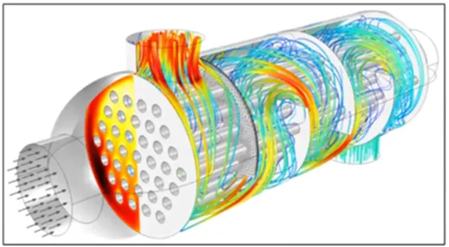
• The word CHT stands for ‘Conjugate heat transfer’.
• CHT analysis is the analysis of heat transfer between a solid and fluid domain by exchanging the thermal energy at interface between them.
• Here the conjugate means there is heat transfer takes place through two modes as conduction and convection simultaneously.
• This analysis is used because whenever thermal energy transfer takes place through 2 modes of heat transfer so we have to simulate and find out the heat transfer coe., maximum temp, avg surface temperature, convective heat transfer coe., conductive heat transfer etc.
• This analysis is generally used in the analysis of heat transfer in exhaust ports, boilers, engines, heat exchangers, regenerators, furnace walls etc.

4. Extended surfaces (Fins) :

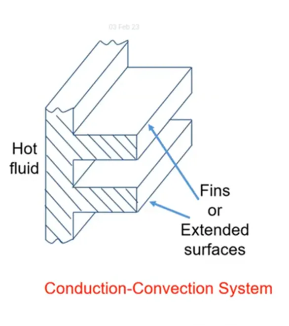
• It is a conduction-convection system employed to dissipate heat from a surface at a faster rate to the surrounding fluids.

Ex : Fined tube in heat exchanger , motorcycle cylinder head, Electronics, air cooled IC engines, Reciprocating air compressors, cars radiators etc.

• Fins are extended surface attached to the primary object to be cooled.
• Heat conducts from primary object into the fins.
• The fin surface provides an extra surface for the heat dissipation to take place via convection.
• Fins can be of different geometries and cross section.
• For mathematical simplicity and wideness of applications, current study will focus on the fins of same cross section throughout the length.

4.1. Types of fins :

1. Longitudinal fin
2. Radial fin
3. Pin fin

4.2. Fin Effectiveness :

• It is a measure of how much heat is conducted by fins as compared to the heat convected from base area without the fin. Mathematically it is given as

εfin=qwith finqw/o fin">` ε fin = q with fin q w/o fin `

Where,

qwith fin=hPKA(To-T∞)">` q with fin = h P K A ( T o - T ∞ ) `

qw/o fin=hA(To-T∞)">` q w/o fin = h A ( T o - T ∞ ) `

Where,

h= conv. Heat transfer coe.

P= perimeter of a fin

K= Thermal conductivity (W/m-K)

A = profile area of a fin or area which is exposed for convection

T_o = surface temp

T_∞ = ambient temp

• Fin effectiveness is improved by using the material with large thermal conductivity.

Ex : gold for electronics, aluminium for motorcycles

• Towards the tip of fin, the temp increases and net potential (T - T_a) reduces.
• High thermal conductivity material also helps keep the fin material near the base temperature, thus maintaining the convective temp gradient equal to the base temp difference (i.e. T_b- T_a).
• The effectiveness also improved by the (P/A) ratio.
• Therefore , thin flat sheets of metal are used as fin.

4.3. Fin efficiency :

• It is defined as the ratio between actual heat transfer rate taking placed through the fin to the max possible heat transfer rate that can occur through the fin i.e. when the entire fin surface is at its root or base temp.
• Mathematically , it is given as

ᶯfin=Actual heat transfer by finIdeal or maximum heat transfer rate from the fin if the entire fin were at base temperature">` ᶯ fin = Actual heat transfer by fin Ideal or maximum heat transfer rate from the fin if the entire fin were at base temperature `fer by finIdeal or maximum heat transfer rate from the fin if the entire fin were at base temperature

i.e. ᶯfin=qfinqidal fin">` ᶯ fin = q fin q idal fin `

where ,

qfin=hPKA(To-T∞)">`q fin = √ h P K A ( T o − T ∞ )`

qidal fin=hA(To-T∞)">`q idal fin = h A ( T o − T ∞ )`

• It can be noted that the fin efficiency increases for lower value of ‘mL’.
• Lower value of ‘mL’ also increases the resistance and thus reduces the overall fin effectiveness.
• Therefore, high efficiency is not always a measured of the high performing fin. Fin effectiveness must also be considered .

Modeling approach :

1. Pre-processing methods :

1.1. Geometry :

• Import the cad model in space-claim.
• Now enabled the share topology

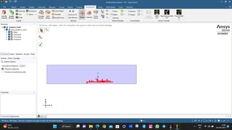
Now we are done with geometry cleanup.

Lets go for meshing.

1.2. Meshing :

• Open mesh

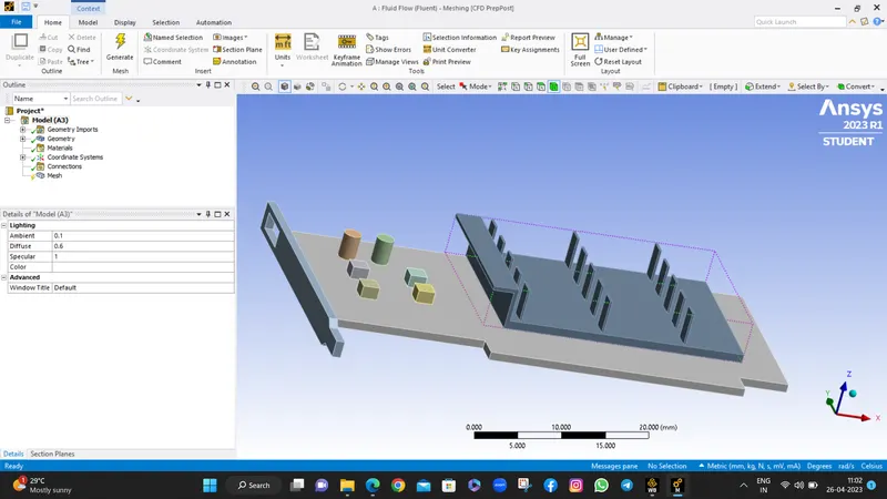
• First of all lets gives the names to the bodies as shown below by selecting appropriate body/face selection method.

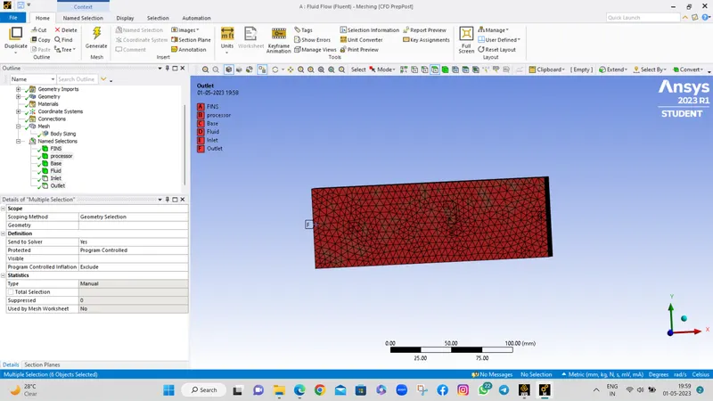
• Now right click on mesh -> generate base line mesh with 5 mm mesh

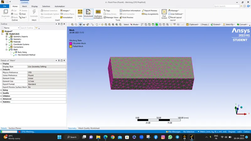
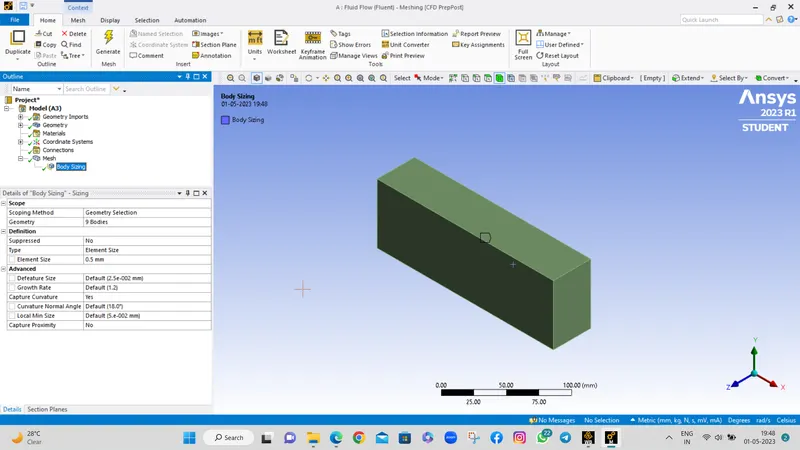
• Now insert sizing select geometry with graphics card witout enclouser.
• For body sizing 0.5 mm mesh elements is generated.

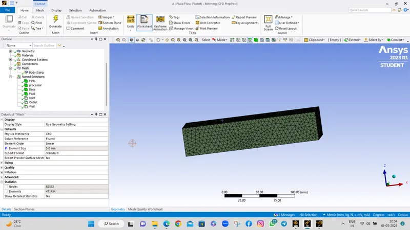
• Total 471452 elements after meshing, with all satisfied quality crieteria.

Now its fine.

Now we are going for setup.

2. Post-procesing methods :

2.1. Setup :

• Open setup i.e. ansys fluent

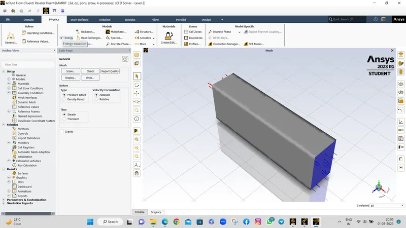
• First here we use parametric command for different cases , In this problem we have to change velocity from 1m/sec to 5 m/sec .
• For that in meshing we have to tick the elements box , so now we have access for parametric.

• Now goto models
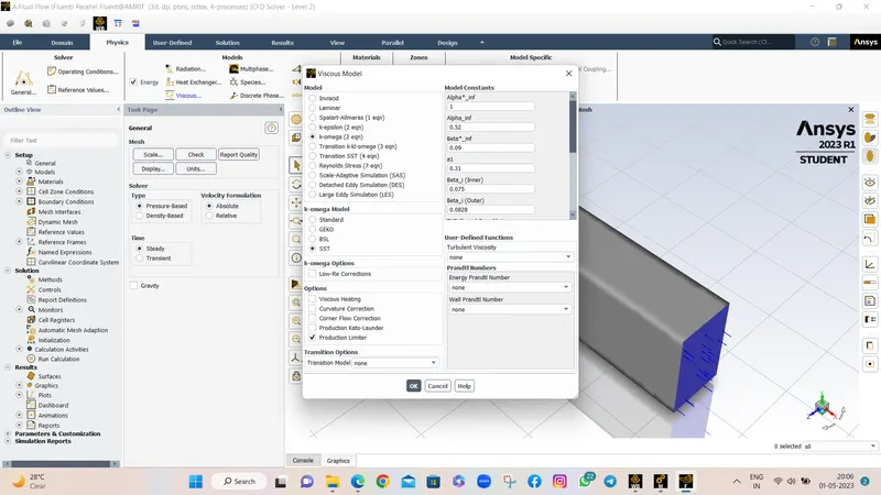
• Enabled energy model and also enabled viscous-K-omega-SST model

• Then goto materials. Now we are creating and assuming following materials

Sr no.	Materials	Density(kg/m3)	Cp(J/kg-K)	K(W/m-K)	viscosity
1	Alumimium(Al)	2719	871	202.4	-
2	Silicon(Si)	2330	712	148	-
3	Ploystyerene(P)	55	1210	0.027	-
4	Air(Fluid)	1.225	1006.43	0.0242	1.78*10^-5

• Now goto cell zones and assign these materials to following parts

Sr. no	Parts	Materials
1	Fluid	Air
2	Fins	Al
3	Processor	Si
4	BODY	p

• Under cell-zone condition enabeled the source terms . now we are assuming that

The heat dissipation by processor= 1W

The size of processor= 8mm x 8mm x 1mm

Volume of processor = 64 mm³= 64 x 10^-9 m³

Therefore heat generated by processor = Heat dissipation by processor volume of processor = 1 64 × 10 - 9

Q_g by processor= 1.5625 x 10^ 7 W/m³

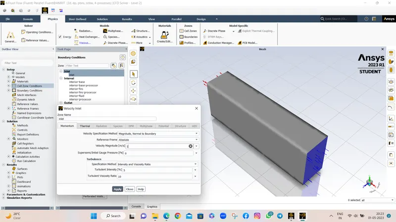
• Now goto boundary conditions and apply as follows

Sr.no	Locations	B.C.s
1	Inlet	Velocity inlet(V=1m/s and T=300K)
2	Outlet	Pressure outlet

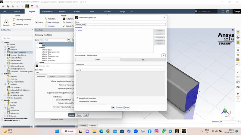
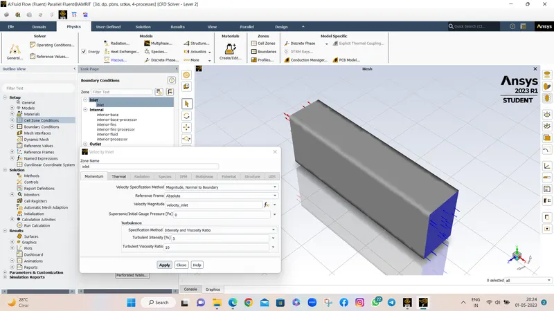
• In bellow enable parameter expression name as velocity_inlet with 1 m/sec .

• Apply coupled method
• Now creates 2 new report definitions as maximum temp and htc at processor
• Now initialize the solution
• Run the simulation for 300 iterations.
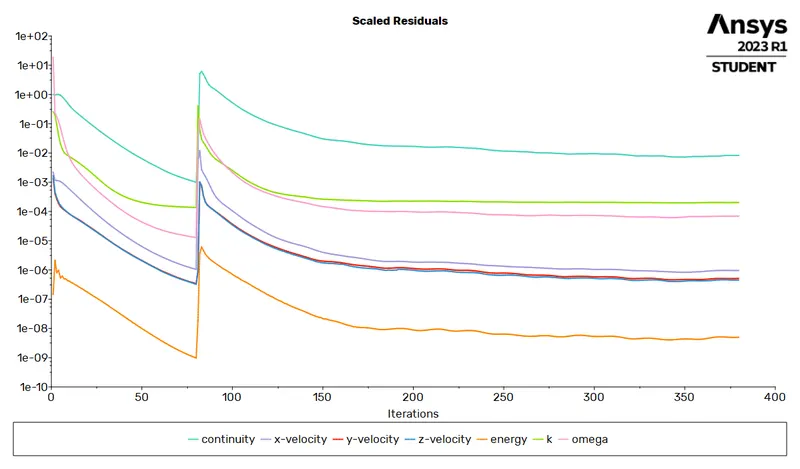
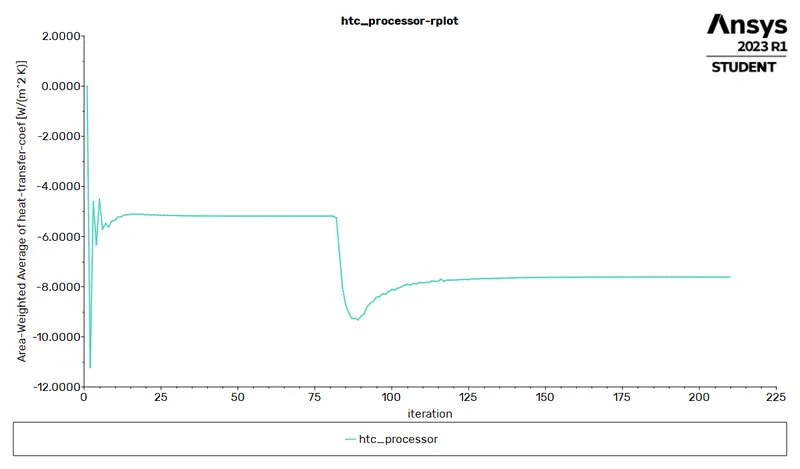
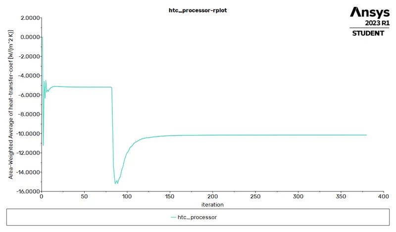
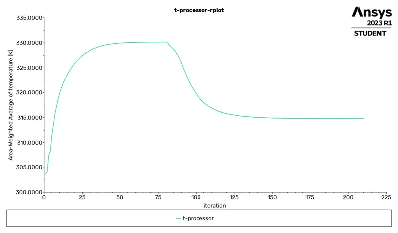
• Lets plot a residual plot, Tmax plot and htc plot.

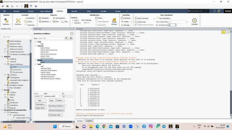
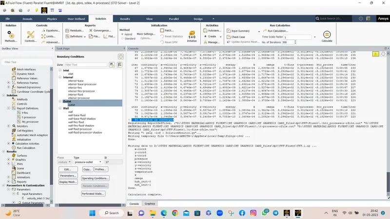
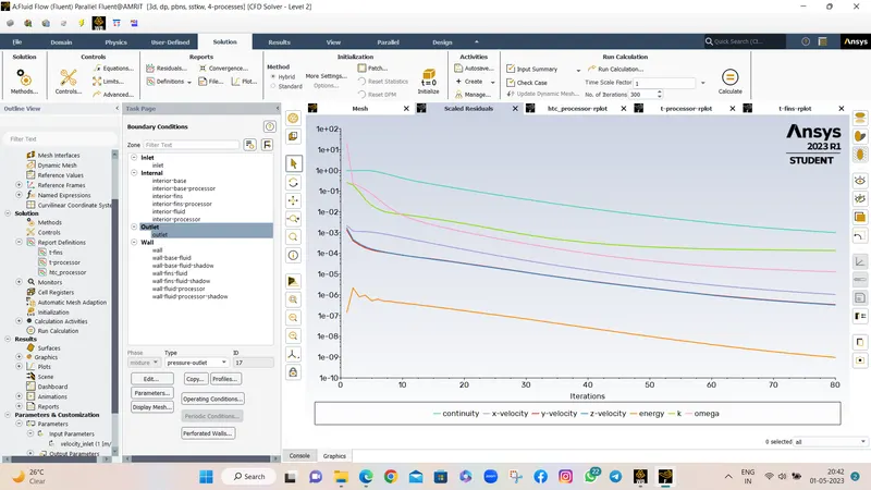
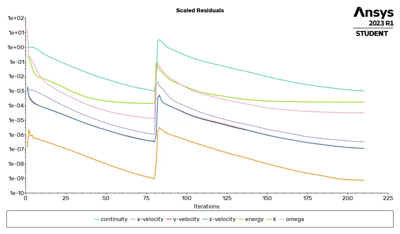
• From above we can said that the solution has been converged means we get constant values after 80 iteration.

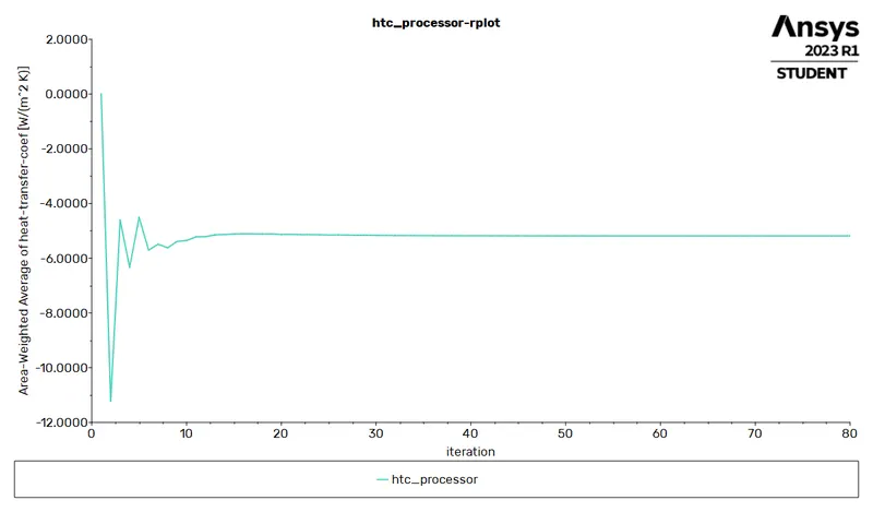
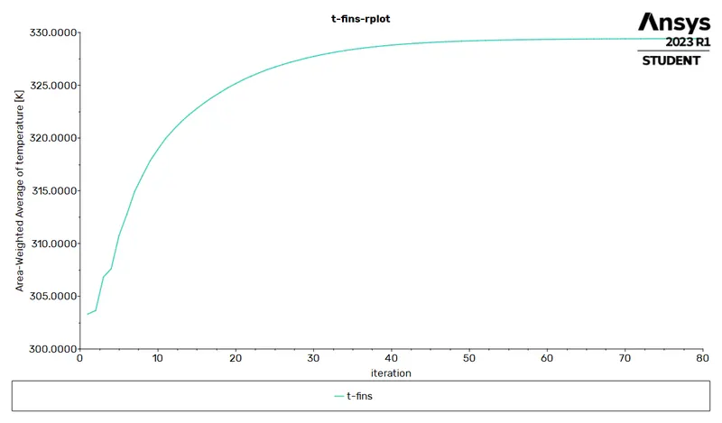
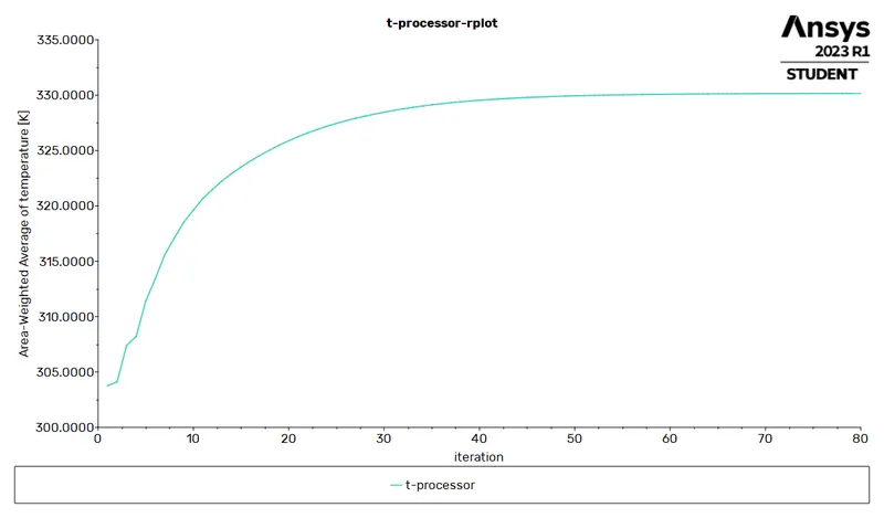
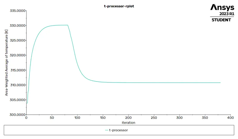
• From above graph we can said that the solution has been converged means we get constant values after some iteration

• Lets goto cfd-post to plot contour plots

2.2. Results :

• Open the cfd-post.
• Plot temp contour plot on graphics card

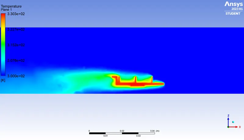
• Now this is a global temp contour plot on a graphics card.

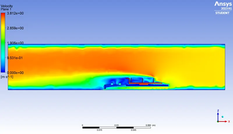
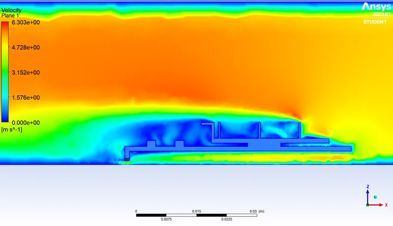
• Lets plot a velocity contour plot on a zx-plane

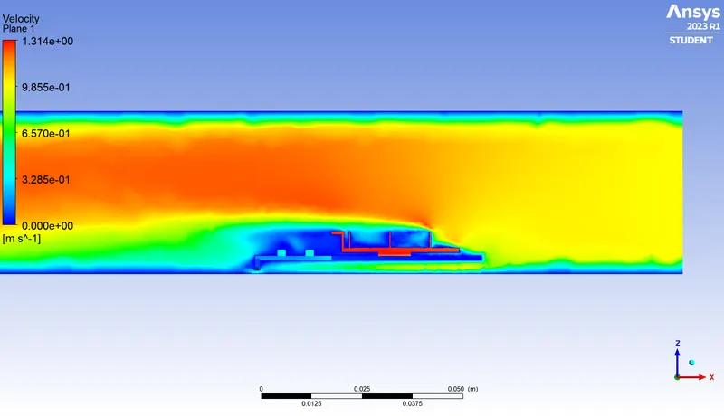
From the velocity contour plot we can see that how the velocity varies when strikes the graphics car

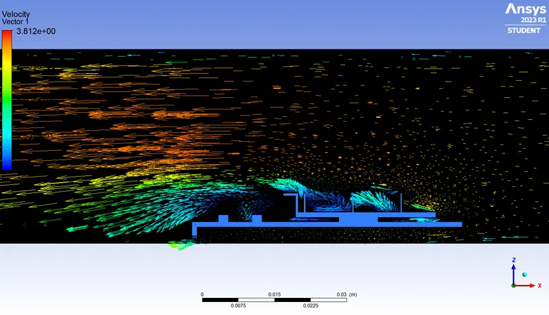
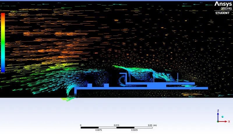
• Lets plot velocity vector plot on zx plane to see wake region

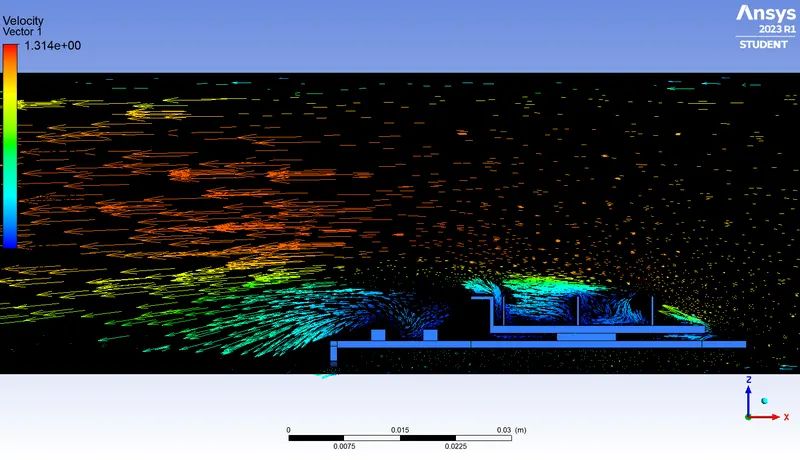
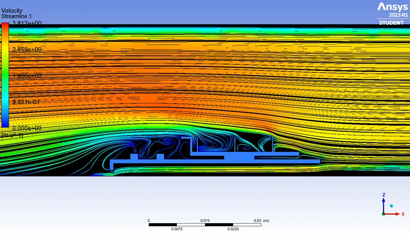
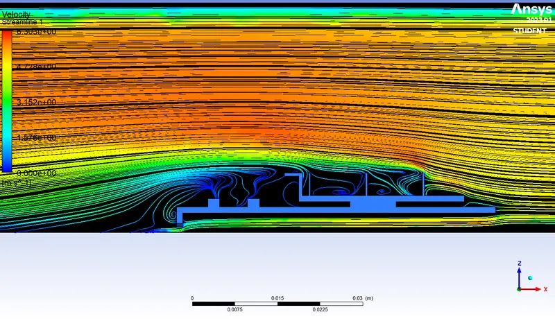
• From this velocity vector plot we can see that how the velocity direction changes and how the wake region or tutbulance

created on graphics card.

• Lets plot velocitystreamline plot on zx plane to see wake region

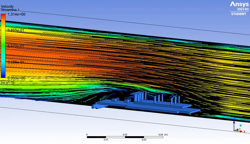
Results :

• Mesh independent study

Sr. no	parameters	Mesh type
1	Cell counts	472542
2	htc(W/m2-K)	-5.1826
3	Tmax(K)	330.16

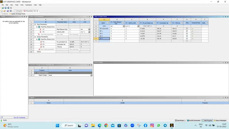
• Htc and tmax for different velocities

Sr. no	Velocity(m/s)	htc(W/m2-K)	Tmax(K)
1	1	-5.1826	330.16
2	3	-7.6163	314.78
	5	-10.156	310.76

• Residual plots

Sr. no	Velocity(m/s)	Residual plots
1	1
2	3
3	5

• Htc plots

Sr. no	Velocity(m/s)	Htc plot
1	1
2	3
3	5

• Temp of Processor plots

Sr. no	Velocity(m/s)	Tmax plot
1	1
2	3
3	5

• Temp contour plots

Sr. no	Velocity(m/s)	Temp contour plots
1	1
2	3
3	5

• Velocity contour plots

Sr. no	Velocity(m/s)	Velocity contour plots
1	1
2	3
3	5

• Velocity vector plots

Sr. no	Velocity(m/s)	Velocity vector plot
1	1
2	3
3	5

• Velocity Streamline Plot

Sr. no	Velocity(m/s)	velocity streamline plot
1	1
2	3
3	5

Conclusions :

1. From 2^nd result we can see that, as the velocity of air at inlet increases, the heat transfer coe. of processor also increases and max temp attained by processor decreases. This happens due to as htc increases more conv. Heat transfer takes place by fluid. From these 3 cases we can conclude that higher the velocity of fluid at inlet more rapidly the processor gets cooled down.

2. From residual plots, Tmax plots, htc plots we can see that the solution gets converged . here as the velocity of fluid increases the number of iterations to get solution converged also increased. Here the convergence means,after some iterations there is no change in the output results or numerical vaues.

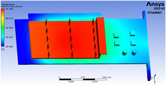
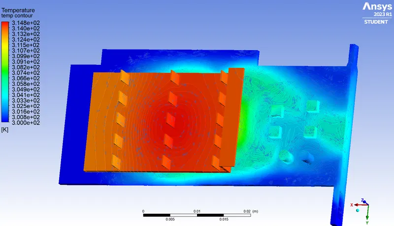
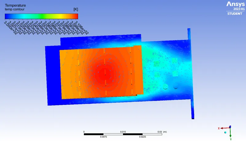
3.From temp contour plots, we can say that, the velocity of air at inlet increases, the surface temp attained by fins gets decreased due to more convective heat transfer takes by fluid.

4.From velocity contour plots and velocity vector plots, we can say that there is more turbulence created by the fluid behind the fins and also wake region area increases which were shown by blue contours.

5.From local temp contour plots, we can see that potential hotspot created by a processor on fins. And this region gets reduced as velocity of fluid increased due to more convective heat transfer takes place. Now this hotspot is developed due to max temp attained by the processor and as max temp attained by processor reduces the hotspot area also reduces.