Week 6 - CHT Analysis on a Graphics card

                  CHT Analysis on a Graphics card

 

Perform a steady-state conjugate heat transfer analysis on a model of a graphics card. You can use appropriate materials of your choice for the simulation. Make sure to properly define the correct solid and fluid zones. Refer the video for further clarification and the model is provided below the video.

Run the simulation for best possible mesh with combination of coarse and refined mesh in different regions. Explain the reason for choosing the particular mesh settings. 

Your Objectives:

1.   Run the simulation by varying the velocity from 1m/sec to 5m/sec for at least 3 velocities and discuss the results.

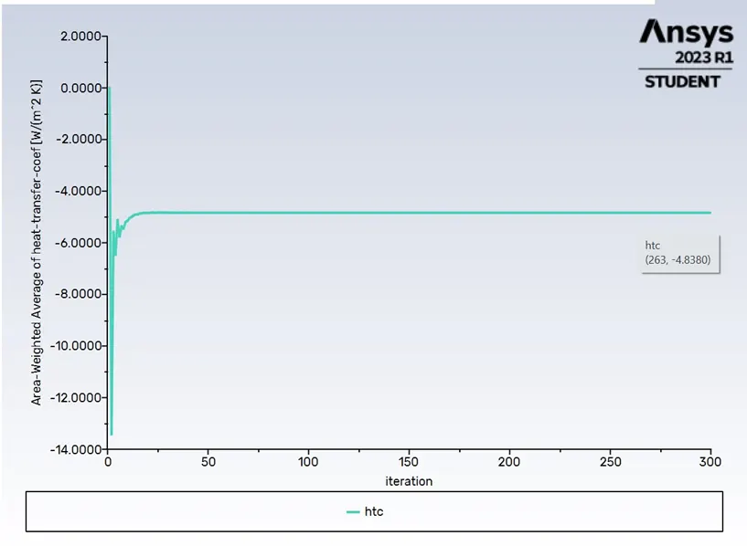
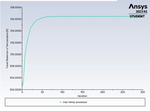
2.   Find out the maximum temperature and heat transfer coefficient attained by the processor.

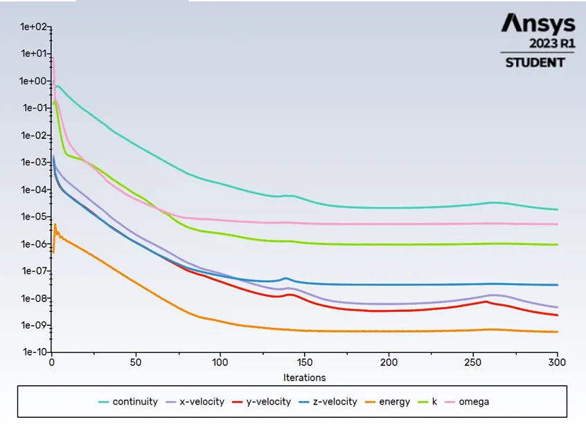
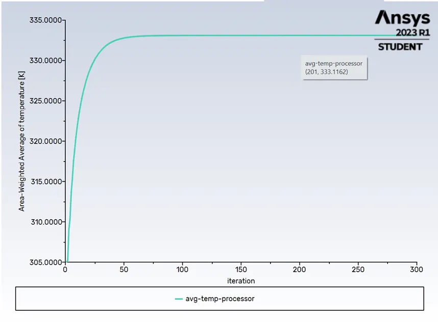
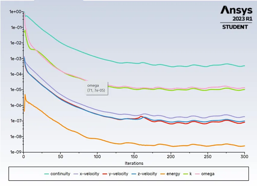
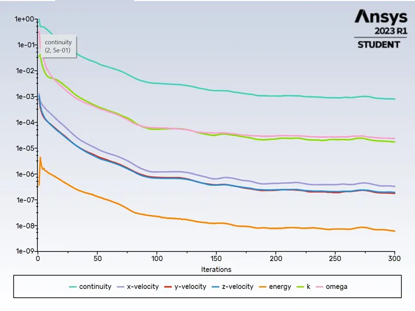
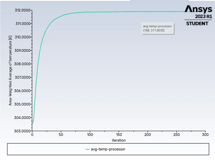
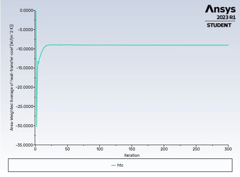
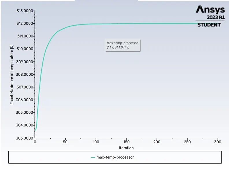
3.   Prove that the simulation has achieved convergence with appropriate images and plots.

4.   Identify potential hotspots on the model.

Aim:

To optimize the thermal performance of a graphics card by accessing temperature distribution, heat transfer mechanism, and priposing design improvements for enchanced cooling and overall performances.

Intoduction for CHT on Graphics card:

Conjugate heat transfer (CHT) analysis for a graphics card involves simulating the simultaneous heat transfer in both solid and fluid regions. The solid region comprises the GPU chip, memory modules, and other electronic components, while the fluid region represents the air or other cooling medium surrounding the graphics card. The goal is to understand how to heat is generated, transferred, and dissipitated within the graphics card assembly.

Setting up the CHT simulation:

1.    Geomentry and Mesh:

 

·    To simulate CHT, youo would start by obtaining a 3D model of the graphics. Proper geomentry preparation and meshing are crucial for accurate results. You’d use finer mesh near heat sources like the GPU chip and memory modules, and coarser mesh in less critical areas. This is because heat generation is concentrated in these regions, requiring a more detailed mesh to capture temperature variations accurately.

2. Materials:

·        Accurate material properties are vital for CHT simulations. Graphics card contain various materials, including metals, plastics, and electronics components, each with its own thermal conductivity and specific heat capacity. These peoperties need to be assigned correctly to ensure realistic results.

3. Boundary conditions:

·        Define boundary conditions to simulate the thermal environment. For the fluid region, you would specify the airflow conditions, such as velocity and temperature. In the solid region, heat sources (eg., Power dissipation from the GPU) and thermal contact conditions between components should be properly defined.

4. Solver and  analysis:

·      Use CHT – capable simulation software (eg., ANSYS, COSMOL, or similar) to set up and solve the CHT problem. The software will use the defined geomentry, mesh, materials, and  boundary conditions to calculate tempratures distributions in both the solid and  fluid regions.

5.   Results and Analysis:

·        After the simulation, analyze the results to understand tempratures profiles, heat fluxes, and thermal gradients within the graphical card. This information can help optimize the design for improved cooling and performance.

Theory of CHT on Graphics Cards:

Conjugate Heat Transfer (CHT) analysis on a graphics cards involves modelling and simulating the simulataneous heat transfer in both solid (the graphics card components) and fluids (the cooling medium, often air) regions. The key theoretical aspects include:

 1.  Heat Transfer Mechanism:

·        CHT accounts for multiple heat transfer mechanisms, such as conduction (within solid components), convection (between solids and fluids), and radiation (if applicable). These mechanisms play a vital role in dissipating heat generated by the graphics card.

2.  Materials Properties:

·        Accurate materials properties, including thermal conductivity and specific heat capacity, are essential. Different materials with graphics card have varying thermal properties, influencing how heat is conducted and stored.

3. Boundary Conditions:

·        Properly defining boundary conditions is critical. In the fluid region, it involves specifying airflow parameters, while in the solid region, heat sources and thermal contacts between components must be considered.

Importance in Practical Applications:

CHT analysis on graphical cards holds significant importance in practical applications for several reasons:

1.  Performance Optimization:

·       Graphics cards are central to various  computing applications, including gaming, rendering scientific simulations, and AI. Efficient thermal management ensures stable and optimal performance by preventing overheating-related throttling.

2.  Reliability and Longevity:

·        Overheating can lead  to premature component failure and reduced graphics card lifespan. CHT  analysis helps design cards that operate within safe temperature limits, enhancing their reliability.

3.   Energy Efficiently:

·        Efficient cooling strategies, informed by CHT simulations, can reduce power consumption by allowing the GPU to operate at lower tempratures, which is crucial in both consumer and data center environments.

4.   Thermal Solutions Development:

·        CHT analysis guides the development of innovative cooling solutions, such as heat sinks, fans, liquid cooling, and improved thermal interfaces, which are essential for next-generation graphics card.

5.   Product Quality Assurance:

·        Ensuring graphics cards remain within thermal specifactions under various conditions is a crucial aspects of product quality assurance. CHT simualtions help verify compliance with these standards.

Solving & Modeling approach:

The solving and modelling approach for a steady-state conjugate heat transfer analysis of a graphics card involves several key steps and techniques.

          1.  Geomentry and Domain portioning:

<!-- [if !supportLists]-->·      <!--[endif]-->Create a 3D model of the graphics card, accurately representing its physical components, such as the Board, Fins and the processor.

<!-- [if !supportLists]-->·      <!--[endif]-->Partition the model into two domains: the solid representing the graphics card components and the fluid domain representing the surrounding air or cooling medium.

2.   Mesh Generations:

<!-- [if !supportLists]-->·      <!--[endif]-->Generate a computational mesh over the entire domain, ensuring that the mesh is fine enough to capture tempratures gradients accurately around heat sources and boundaries. Use techniques like structured meshing depending on the geomentry complexity.

3.   Material Properties:

<!-- [if !supportLists]-->·      <!--[endif]-->Assign appropriate material properties to both the solid and fluid domains. Define thermal conductivity, specific heat capacity, and density for solid components and properties like air density, thermal conductivity, specific capacity, and dynamic viscosity for the fluid domain.

 

4.   Boundary Conditions:

<!-- [if !supportLists]-->·      <!--[endif]-->Define boundary conditions that describe the interaction between the graphics card and its environment. This includes specifying inlet conditions for fluid flow ( e.g., velocity, temperature) and heat sources within the solid components (e.g., power dissipitation by the processor).

          5.   Conjugate Heat Transfer Modeling:

<!-- [if !supportLists]-->·      <!--[endif]-->Implement a conjugate heat transfer model to account for heat exchange between the solid and fluid domains. This involves setting up appropriate heat transfer  coefficients or using models that describe heat transfer across the interface between the two domains.

6.   Solver Configuration:

<!-- [if !supportLists]-->·      <!--[endif]-->Configure the numerical solver for the simulation. Specify that it is a  steady-state analysis, set convergence criteria, and choose turbulence models if simulating fluid flow. Adjust solver setting for efficiency and accuracy.

7.   Running Simulations:

<!-- [if !supportLists]-->·      <!--[endif]-->Perform the simulations for various operating conditions, such as different airflow velocities (e.g., 1 m/s, 2 m/s, 3 m/s, 5 m/s) as specified. The solver iteratively calculates tempratures distributions until convergence is achieved for each condition.

8.   Post-Processing and Analysis:

<!-- [if !supportLists]-->·      <!--[endif]-->Analyze simulations  results to extract important information,

<!-- [if !supportLists]-->·      <!--[endif]-->Determine the maximum processor temperature to access thermal performance.

<!-- [if !supportLists]-->·      <!--[endif]-->Calculate heat transfer coefficients at various locations to evaluate cooling efficiency.

<!-- [if !supportLists]-->·      <!--[endif]-->Identify regions with elevated tempratures to pinpoint potential hotspots.

<!-- [if !supportLists]-->·      <!--[endif]-->Generate tempratures profiles, velocity fields, and heat transfer maps to visualize the thermal behavior within the graphics card.

1. Geomentry:

·        Open SpaceClaim.

·        Import the Geomentry in SpaceClaim.

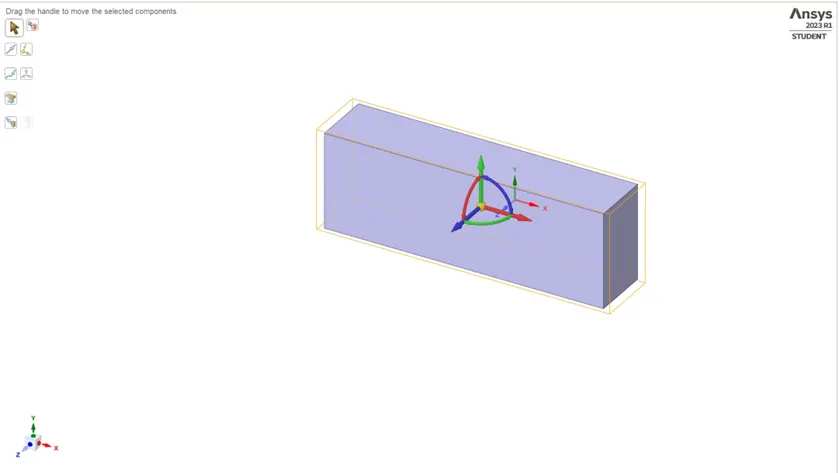
·         Here the geomentry has been loaded to SpaceClaim

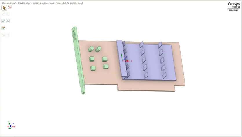
·        Separate component name has been created for the different parts of the graphics card as base, processor, fins and enclosure.

·        The enclosure represents the fluid domain over which the flow of air given as intake with specific velocity.

·        Now prepare the object to a shareto opology.

 

Shareto opology :

·       The shareto opology is used to find the edges.

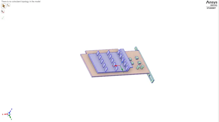
·      Enabling Shareto opology,

·      By clicking it, it will identify the edges between them.

·      After the Shareto opology the surfaces are been checked and can be interconnect to the surfaces.

  2. Meshing:

For meshing we open Meshing, where we mesh our model so that we can use it to solve our model.

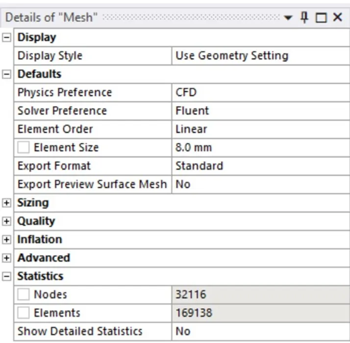
Case 1Baseline Mesh

·      Base Mesh Size – 8.0mm

·      Number of elements – 169138

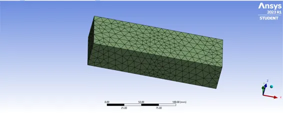
·      Here the mesh has been updated

 

 

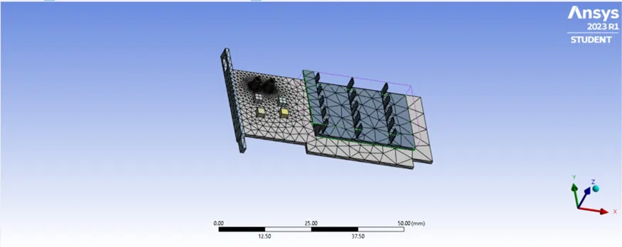
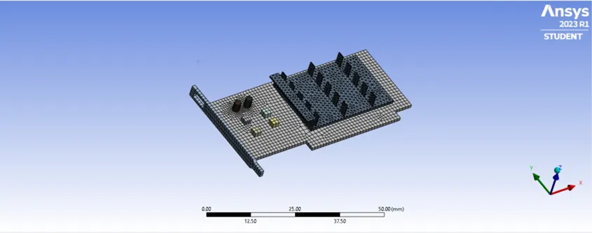
·      The baseline mesh of 8.0mm has been updated.

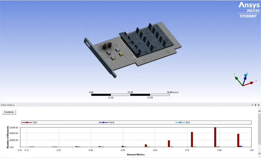
·      This plot shows the quality of the Baseline Mesh.

·      Hide the enclosure to get the complete view of graphics card.

Named Selections:

·       Naming the surfaces helps identify the mesh.

  Inlet:

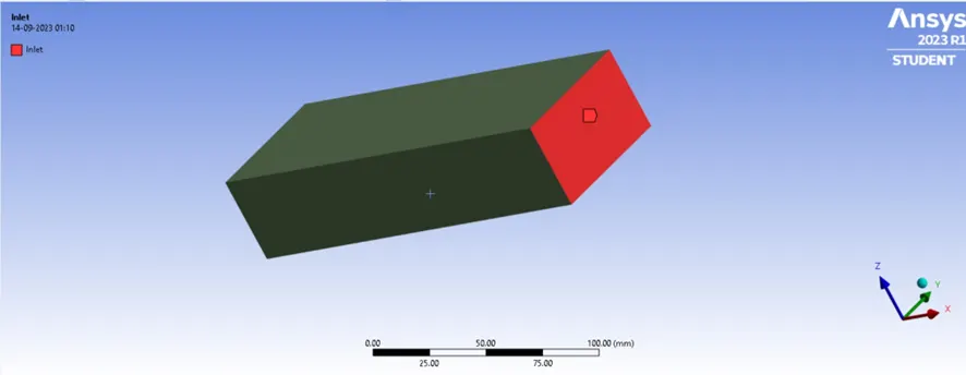
·      This represents the Inlet of the Mesh.

 

Outlet:

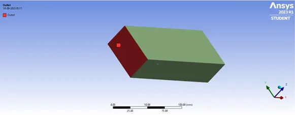
·      This represents the Outlet of the Mesh.

Symmentry:

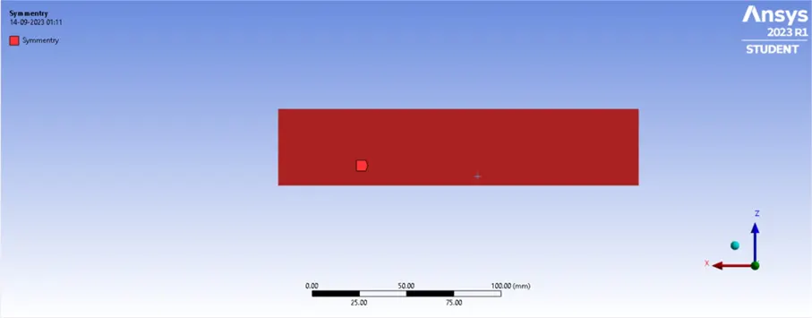
·      This represents the Symmentry of the Mesh.

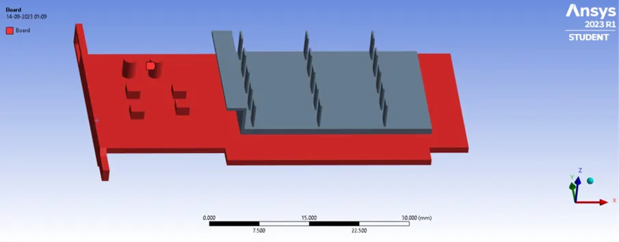
Board:

 

  Fins:

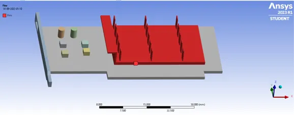
Processor:

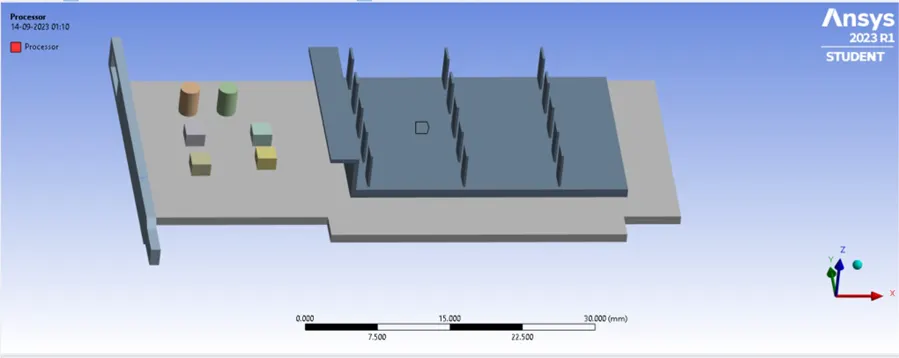
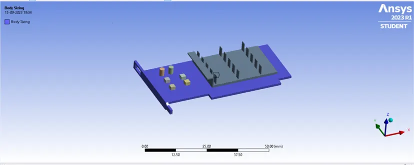
Body sizing:

·      Click on mesh à Body Sizing

·      Select base mesh and provide sizing of 1mm and updated.

 

Processor and Fins:

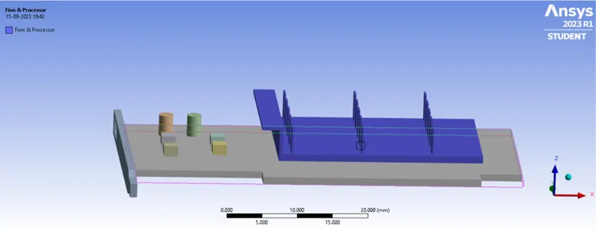
·      The size of Fins and Processor is 1mm

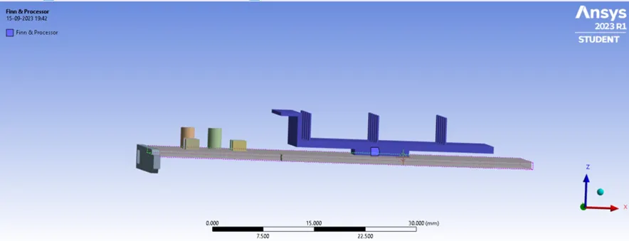
·      Generate the mesh, the refinement is complete and next update the mesh pattern.

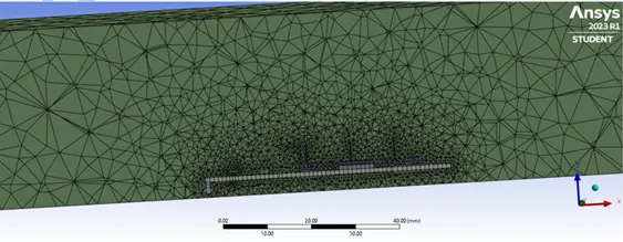
·      Enable show all bodies option to view the surfaces.

·      This plot represents the cross sectional of the mesh.

·      Now the mesh is ready to run for the simulation.

 

3. Set-up:

The mesh have been updated in the set-up.

1. General:

·    Time            - Transient Enabled

2.  Viscous Model       -  k - epsilon

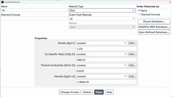
Now since it is a conjugate heat transfer, so different materials are assigned at different zones.

3.  Energy equation – It has been Enabled.

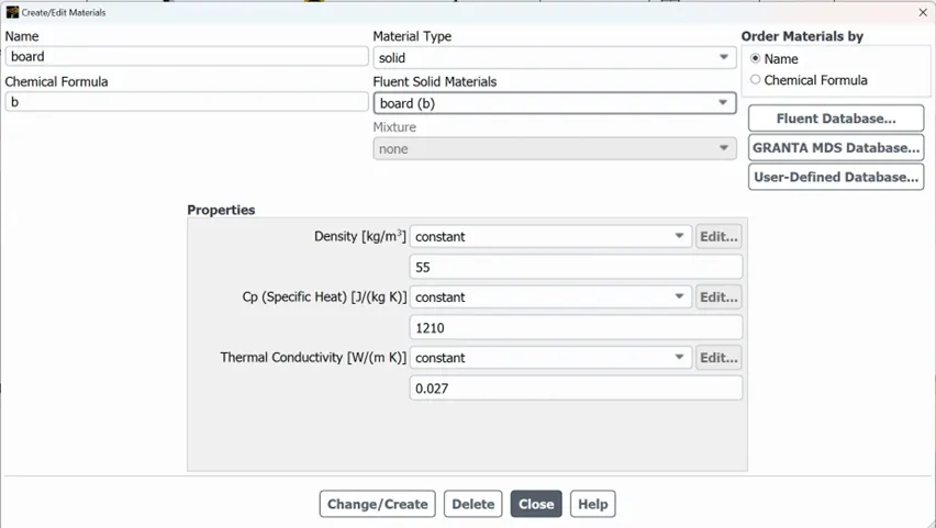
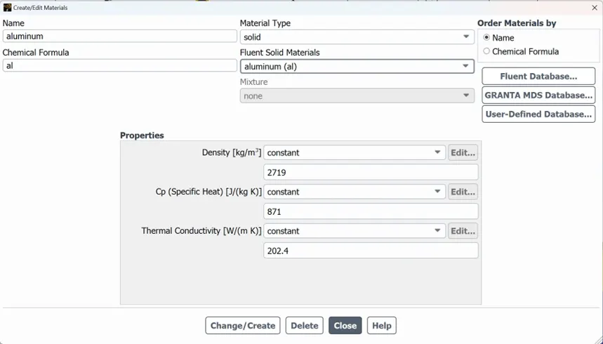
4. Material Properties - Solid

          Silicon

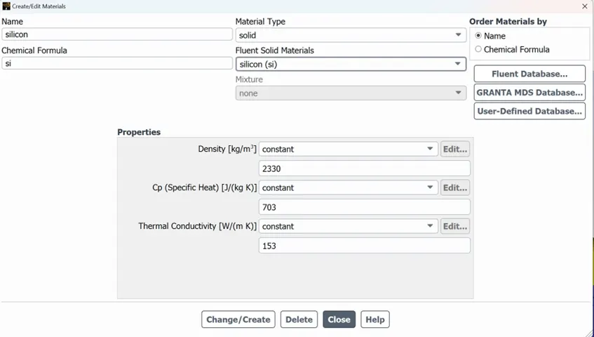
Board

Aluminium

Air

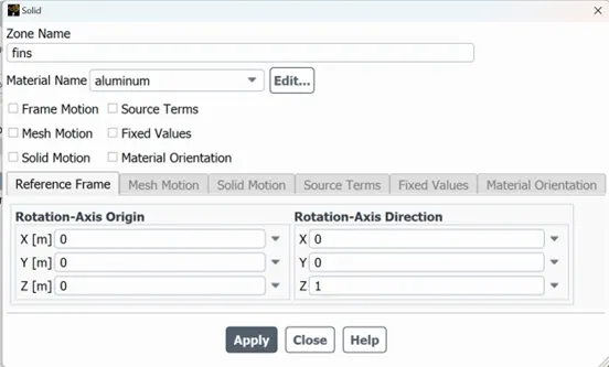
5. Cell Zones Conditions

Solid - Processor

Type – Solid

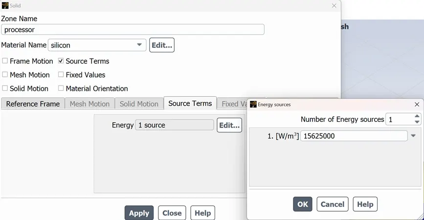
·      Here we have taken a graphic card processor as 1w.

·      Volume of processor = 8*8*1 = 64mm^3 = 64 x 10^9 m^3

·      Hence heat generated =  1/(64 x 10^9) = 15625000 w/m^3

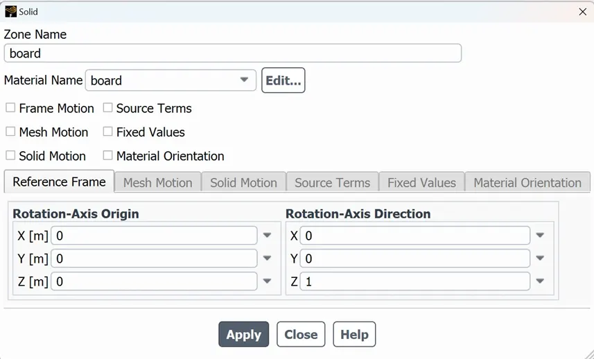
Type – Board

Type – Fins

 

 6. Boundary Conditions:

The boundary condition is to provide the input physics parameter à go to boundaries à select inlet and specify the inlet air velocity as per required.

Inlet

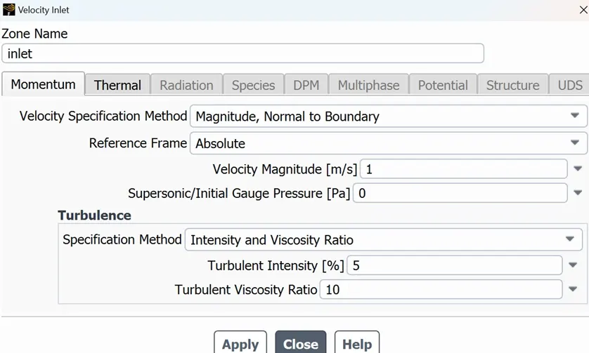
·    The thermal temperature of the Velocity inlet – 300k

·     Set the wall to adiabatic conditions and symmentry walls to  symmentry.

 

Outlet

·   Temprature – 300k

· Keep the boundary conditions of interior wall to coupled phase, as there is fluid and solid interaction.

 

7.  Initilization:

o   Hybrid Initilization

8.   Run calculations:

·   No of Iterations – 300

Residuals

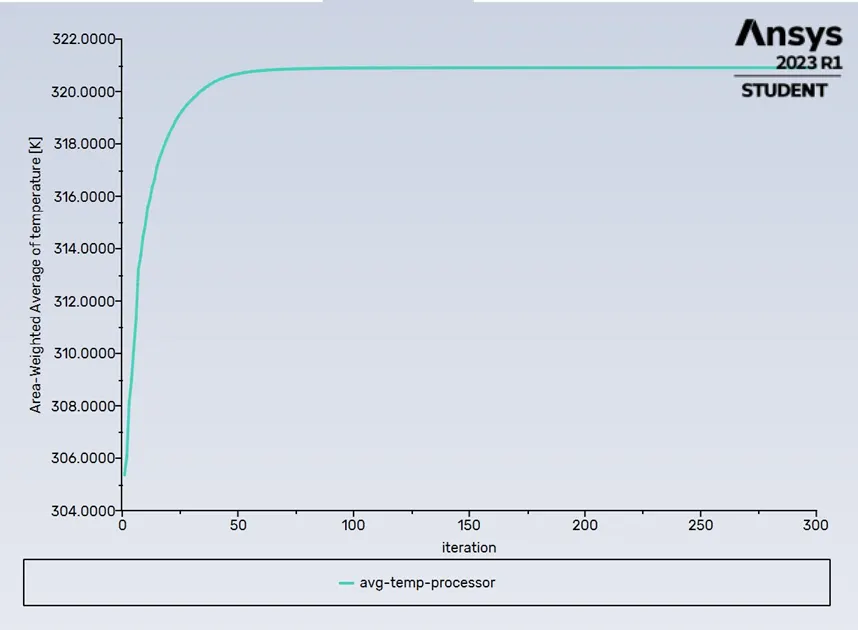
  Area Weighted Average of Temprature:

 

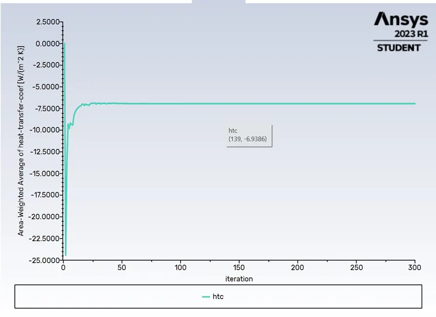
Area Weighted Average of heat transfer Co-efficient:

 

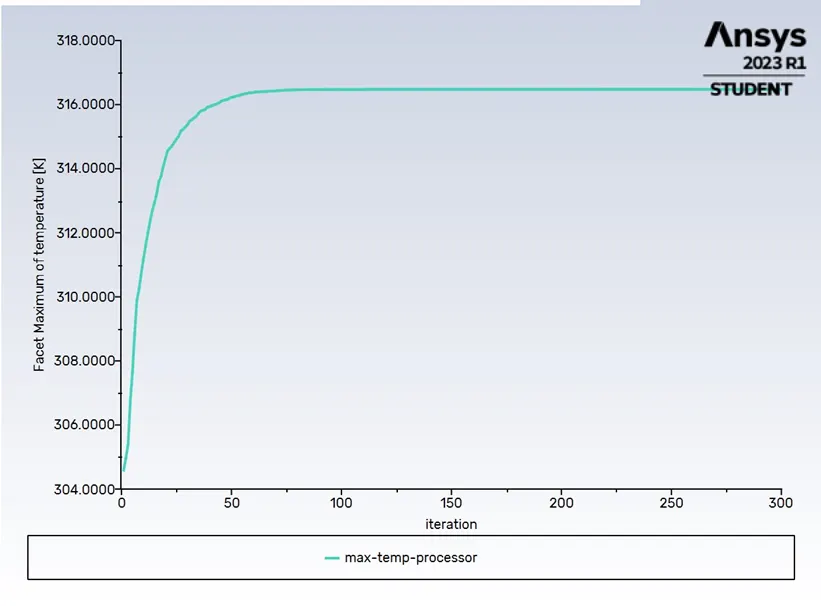
Facet Maximum of temperature:

 

 Results:

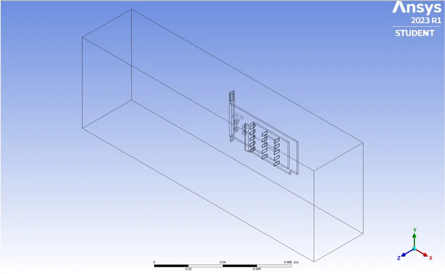
·    The plot shows the wireframe of the surface model has been updated in post-processing results.

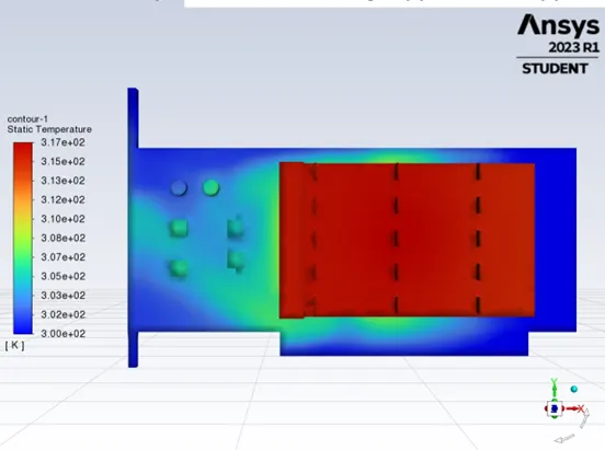
Temprature plane:

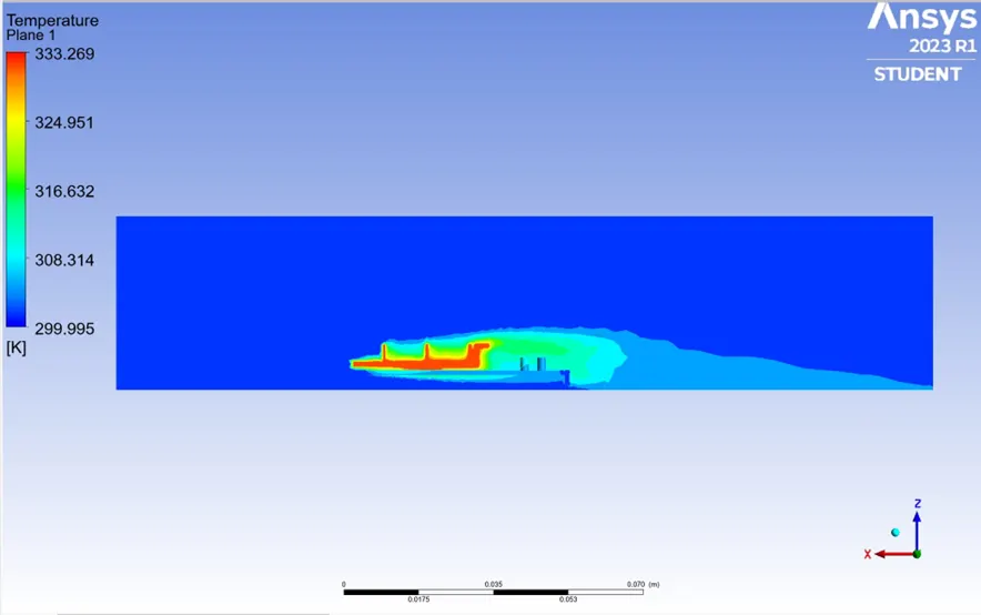
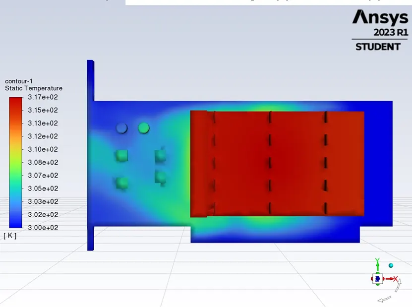
·            This plot shows the temperature of the contour.

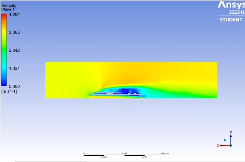
Velocity Plane:

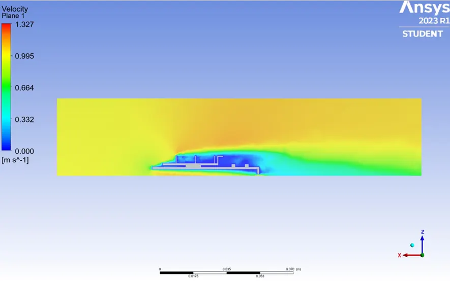
·        This plot shows the velocity on the contour.

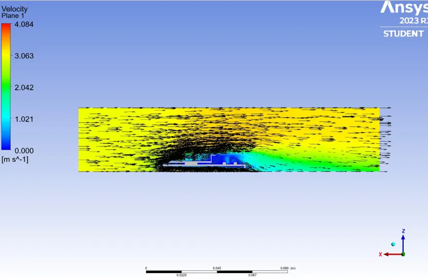
Velocity Vector:

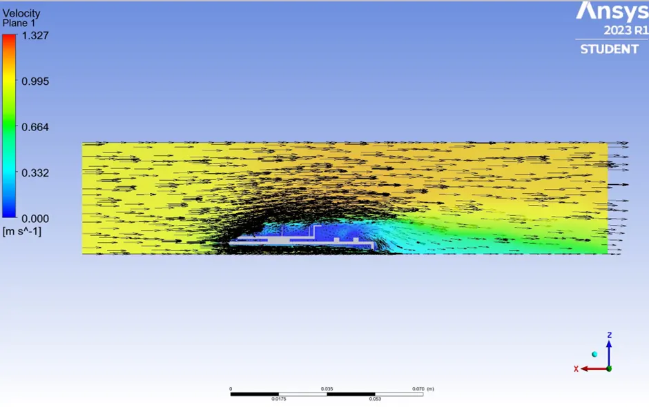
·     This plot shows the Vector among the plane.

Case 2 Refined Mesh

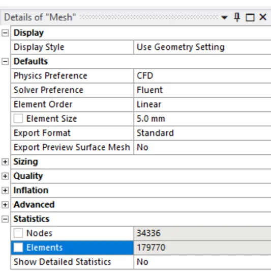
·      Base Mesh Size – 5.0mm

·      Number of elements – 179770

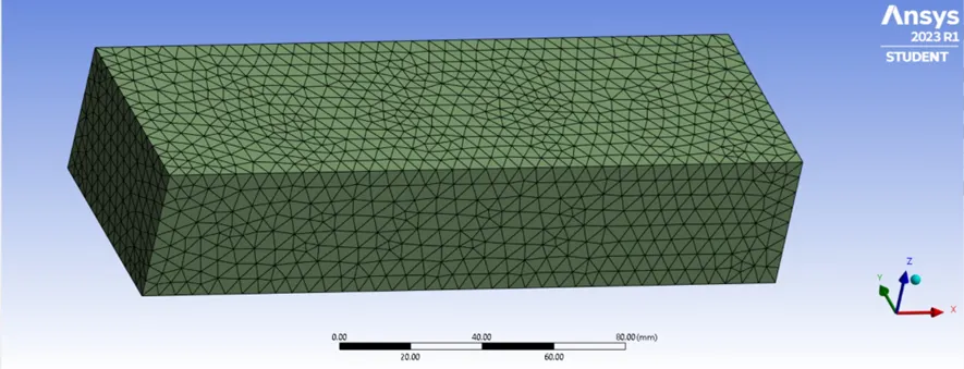
·      Here the Refined mesh has been updated to 5.0 mm

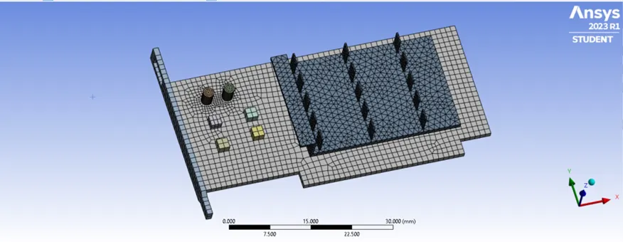
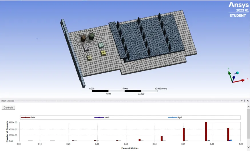
·      This plot shows the quality of the Baseline Mesh.

·      Hide the enclosure to get the complete view of graphics card.

Set-up:

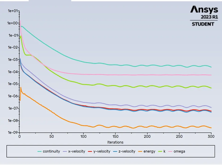
Residuals:

·     No of Iterations – 300K

·     Velocity – 2 m/s

Area Weighted Average of Temprature:

Area Weighted Average of heat transfer Co-efficient:

Facet Maximum of temperature:

 

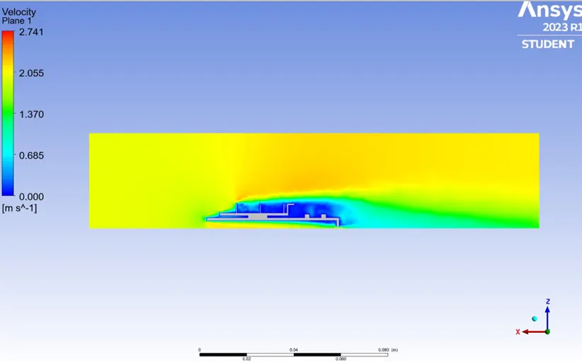
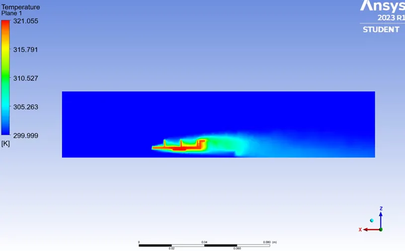
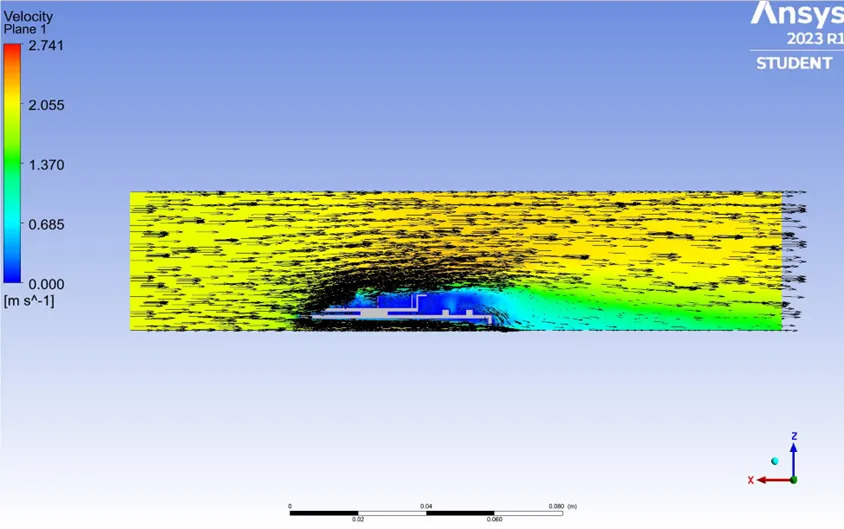
Results:

Velocity Plane:

 

Temprature Plane:

 

Velocity Vector:

 

Case 3

·      Base Mesh Size – 8.0mm

·      Number of elements – 169107

Residuals:

·      No of Iterations – 300K

·      Velocity – 3 m/s

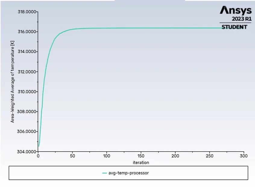
Area Weighted Average of Temprature:

 

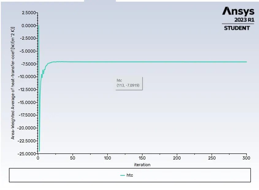
Area Weighted Average of heat transfer Co-efficient:

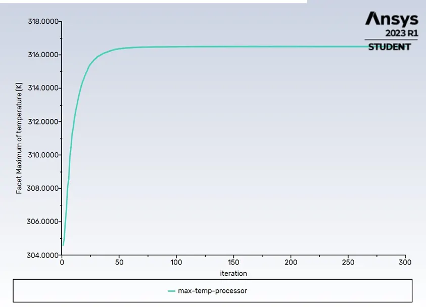
Facet Maximum of temperature:

Results:

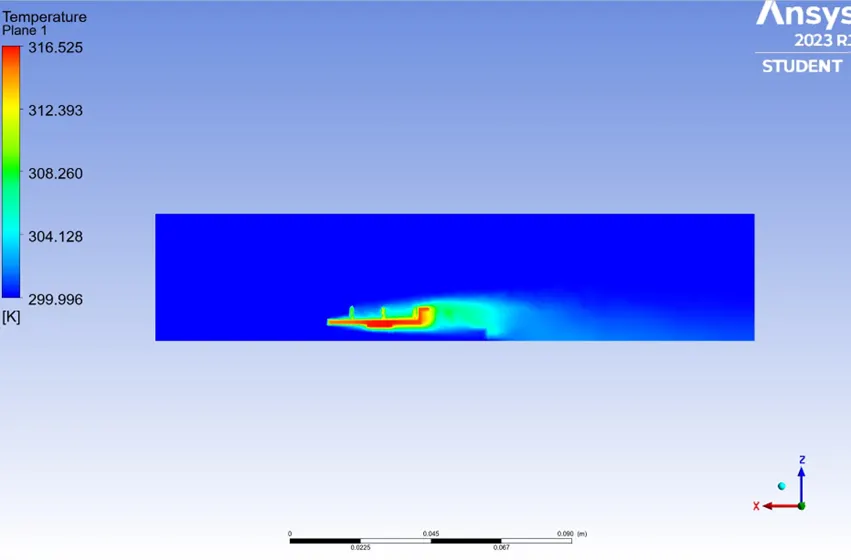
Temprature Plane:

Velocity Plane:

Velocity Vector:

 

Case 4

·      Base Mesh Size – 8.0mm

·      Number of elements – 169107

                Residuals:

·      No of Iterations – 300K

·      Velocity – 5 m/s

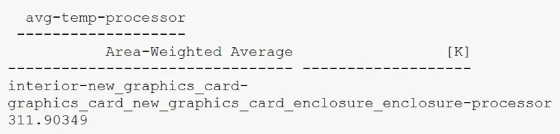
Area Weighted Average of Temprature:

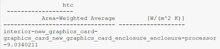
Area Weighted Average of heat transfer Co-efficient:

Facet Maximum of temperature:

 

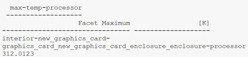
Results:

Temprature Plane:

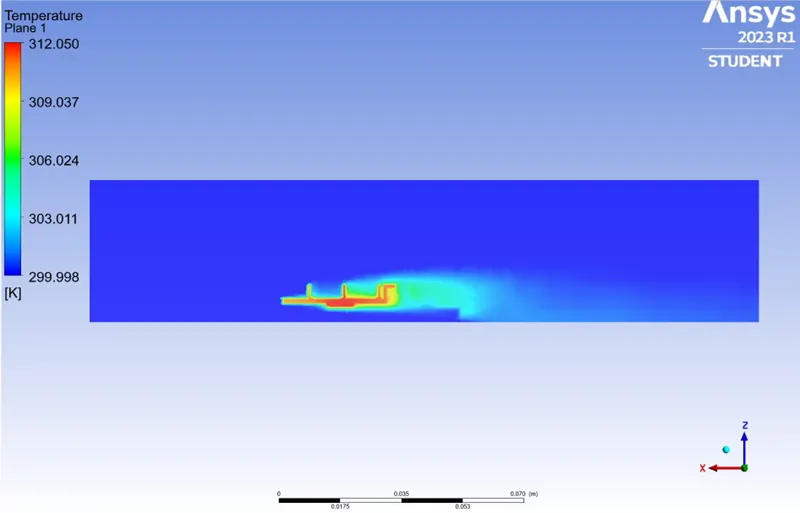
Velocity Plane:

 

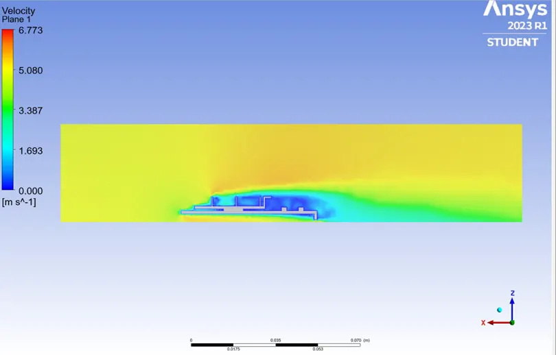
Velocity Vector:

 

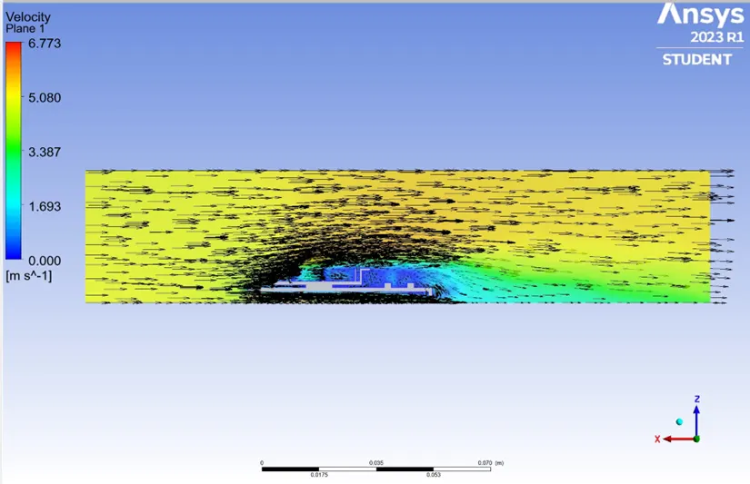
Inlet velocity      (m/s)	Temprature of processor (K)	Heat transfer coefficient	Maximum Predicted velocity
Case 1 -  ( Baseline Mesh) Velocity 1 m/s	333.11861	-4.8379738	333.24234
Case 2-  ( Refined Mesh)  (Velocity 2 m/s)	320.90797	- 5.76199	321.02194
Case 3  (Velocity 3 m/s)	316.37487	-7.0933501	316.49405
Case 4 (Velocity 5 m/s)	311.90349	-9.0340211	312.0123

 

Conclusion:

In this study, a comprehensive steady-state conjugate heat transfer analysis of a graphics card was conducted. The following key findings and conclusions were drawn:

Firstly, we observed a notable variation in the graphics card’s thermal performance as we increased the airflow velocity, ranging from 1 m/s, 2m/s, 3m/s and 5 m/s. Specifically, as the airflow velocity rose, we witnessed a corresponding improvement manifested as a reduction in the maximum processor tempratures, indicating enchanced cooling efficiency with higher airflow velocities.

Furthermore, our analysis successfully identified specific areas on the graphics card where tempratures were significally elevated. These identified regions represent potential hotspots that require particular attention during the design phase to ensure effective cooling solutions.

We also determined heat transfer coefficients at various locations on the graphics card. These coefficients provide valuable insights into the efficiency of heat dissipation and can serve as crucial guidance for optimizing heat sink and fan configurates, ultimately enhancing cooling performance.

The convergence of our simulation results was confirmed through the stability of the temperature field over time. This convergence assures the reliability of the obtained results, reinforcing their validity and applicability to real-world scenerios.

Finally, this study underscored clear opportunities for improving the graphics card’ thermal performance. Adjustments to cooling system parameters, such as fan speed and heat sink design, can effectively mitigate hotspots and elevate overall cooling efficiency.

In summary, our conjugate heat transfer analysis has provided valuable insights into the thermal behavior of the graphics card under varying airflow conditions. These findings are instrunments in informing design enhancements and contributing to the development of more efficient and dependable graphic card in the future. Nonetheless, it’s essential to acknowledge that the accuracy of this analysis is contigent on factors like material properties, boundary conditions, and modelling assumptions, and further refinement may be necessary for precise thermal predictions in practical applications.